Lesson 8: Modeling with Sine Functions

Objectives

Given a parameterized sine function, describe how it changes as each parameter is adjusted.
Given a plot of data, determine whether a sine function is appropriate.
Given data exhibiting a sinusoidal relationship, approximate the parameters by hand.
In R, use fitModel() to obtain the best-fit sine model.
Evaluate a sine model at a given input and interpret the answer.

TemperaturesDanville dataset

The TemperaturesDanville dataset, in the MMAC package, records the average maximum temperature in Danville, Kentucky, at the beginning of each month since January 2006. It has 60 rows. The variable Month counts months from January 2006 and runs 0 to 59. The variable Temperature is in degrees Fahrenheit and runs 33.6 to 92.3.

Sine Explorer Open full screen

1. Parameters of a Sine Model

Objective. Given a parameterized sine function, describe how it changes as each parameter is adjusted.

Definition 1 (Sine model).

A sine model has the general form

y = A\sin\!\left(\frac{2\pi}{P}(x - h)\right) + v,

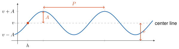
with four parameters: the amplitude $A$ , the period $P$ , the horizontal shift $h$ , and the vertical shift $v$ . The amplitude and the period are positive: $A > 0$ and $P > 0$ .

The function $y = x\sin(x)$ is not a sine model, because the factor in front of the sine is $x$ , which changes with the input, and the definition requires a constant amplitude $A$ . Its peaks grow taller as $x$ moves away from 0 in either direction.

The amplitude $A$ is half the distance between the maximum and the minimum output values of the sine function. Increasing $A$ raises the peaks and deepens the troughs.

The period $P$ is the length of the smallest input interval needed for the sine function to complete an entire oscillation. Increasing $P$ stretches the curve horizontally.

The vertical shift $v$ is the height of the output that is halfway between the maximum and the minimum output values of the sine function. The curve oscillates about the center line $y = v$ . Increasing $v$ slides the whole curve up.

The horizontal shift $h$ is the first input $x = h$ at or to the right of $x = 0$ at which the sine function is increasing and its output equals the vertical shift $v$ . Increasing $h$ slides the whole curve to the right.

Since $A > 0$ , the two extreme outputs come from the amplitude and the vertical shift:

\text{maximum} = v + A, \qquad \text{minimum} = v - A.

Axis of each parameter. The amplitude $A$ and the vertical shift $v$ are measured on the vertical axis. The amplitude is a distance between outputs, and the vertical shift is an output value. The period $P$ and the horizontal shift $h$ are measured on the horizontal axis. The period is a distance between inputs, and the horizontal shift is an input value.

Radians. R’s sin() takes radians (Lesson 1 sheet, section 2). A calculator in degree mode gives a different value: $\sin(2)$ is about 0.035 in degree mode and about 0.909 in radians.

Lowest nonnegative horizontal shift. Because a sine curve crosses its center line while increasing once every period, each of $h$ , $h + P$ , $h - P$ , and every whole-period translation gives the same curve. The lowest nonnegative horizontal shift is the one value of $h$ that satisfies $0 \le h < P$ , reached by adding or subtracting whole periods.

Parameters in Desmos. Type the general form at desmos.com/calculator with $A$ , $P$ , $h$ , and $v$ as letters, and Desmos adds a slider for each parameter. Start from $y = \sin(x)$ . Moving one slider at a time shows which feature of the curve each parameter controls.

Example 1

Give $A$ , $P$ , $h$ , and $v$ for the function below, and give its maximum and minimum outputs:

y = 5\sin\!\left(\frac{2\pi}{3}(x - 2)\right) + 8.

ShowHide solution

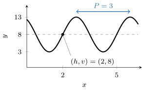
By the definition of a sine model, the function has the general form $y = A\sin\!\left(\frac{2\pi}{P}(x - h)\right) + v$ . Matching it term by term gives $A = 5$ , $P = 3$ , $h = 2$ , and $v = 8$ . The extreme outputs are

\text{maximum} = v + A = 8 + 5 = 13, \qquad \text{minimum} = v - A = 8 - 5 = 3.

On the graph, the curve crosses its center line $y = v = 8$ while increasing at the point $(h, v) = (2, 8)$ . It rises to the maximum 13, falls to the minimum 3, and repeats every $P = 3$ units of input, the distance between the two peaks.

Example 2

Give the lowest nonnegative horizontal shift for the function below, and rewrite the function with it:

y = 2\sin\!\left(\frac{2\pi}{4}(x + 1)\right) + 3.

ShowHide solution

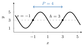
Since $x + 1 = x - (-1)$ , the function crosses its center line $y = 3$ while increasing at $x = -1$ , which lies left of $x = 0$ . The period is $P = 4$ . The next crossing while increasing is one period later, and it satisfies $0 \le h < 4$ :

h = -1 + 4 = 3.

The given function equals

y = 2\sin\!\left(\frac{2\pi}{4}(x - 3)\right) + 3.

On the graph, the two marked points are the crossings while increasing at $x = -1$ and at $h = 3$ , one period $P = 4$ apart. Both values of $h$ in the general form give the same curve.

Example 3

Each function below differs from $f(x) = \sin(x)$ in exactly one parameter. Name the parameter, give its new value, and describe how the graph changes:

g(x) = \sin(x - 2), \qquad k(x) = 4\sin(x), \qquad m(x) = \sin(x) + 2, \qquad n(x) = \sin(2x).

ShowHide solution

In the general form, $f(x) = \sin(x)$ has $A = 1$ , $P = 2\pi$ , $h = 0$ , and $v = 0$ , because the coefficient of $x$ is 1, and $\frac{2\pi}{P} = 1$ gives $P = 2\pi$ . Define the five functions and plot them on one set of axes, each changed function in its own color:

f = makeFun(sin(x) ~ x)
g = makeFun(sin(x - 2) ~ x)
k = makeFun(4*sin(x) ~ x)
m = makeFun(sin(x) + 2 ~ x)
n = makeFun(sin(2*x) ~ x)
plotFun(f(x) ~ x, xlim = range(-10, 10), ylim = c(-8, 8))
mathaxis.on()
plotFun(g(x) ~ x, add = TRUE, col = "tomato3")
plotFun(k(x) ~ x, add = TRUE, col = "turquoise3")
plotFun(m(x) ~ x, add = TRUE, col = "purple3")
plotFun(n(x) ~ x, add = TRUE, col = "orange2")

The four panels below show the changes one at a time, with $f$ in dark blue and the changed function in red.

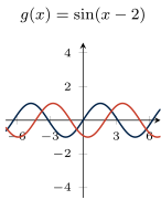
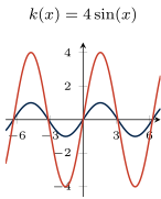
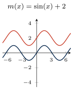
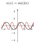
The function $g$ changes the horizontal shift: $h = 2$ . The curve slides 2 units to the right. The period and the center line stay the same.
The function $k$ changes the amplitude: $A = 4$ . The peaks rise to 4 and the troughs fall to $-4$ . The period and the center line stay the same.
The function $m$ changes the vertical shift: $v = 2$ . The peaks, the troughs, and the center line rise by 2. The period and the amplitude stay the same.
The function $n$ changes the period: $P = \pi$ , because $\frac{2\pi}{P} = 2$ . The peaks sit half as far apart as the peaks of $f$ . The center line and the amplitude stay the same.

Next: 2. Appropriateness of a Sine Model Lesson map

2. Appropriateness of a Sine Model

Objective. Given a plot of data, determine whether a sine function is appropriate.

Definition 2 (Sinusoidal data).

Sinusoidal data are data whose outputs rise and fall in the shape of a sine curve, between two roughly constant extremes, repeating at a roughly constant input spacing.

Daily high temperatures from January to June rise and fall from day to day, while both the highs and the lows climb toward summer. Those data are not sinusoidal, because the definition requires two roughly constant extremes.

Decide from the standard plot whether a sine model is reasonable, because a semi-log or log-log plot of an oscillation still oscillates. Many oscillating quantities also reach zero or go below it, and at those outputs log() returns -Inf or NaN.

Evidence of repetition. Repetition shows on the plot when the data cover more than one cycle. A single cycle is enough when the quantity is known to repeat. Sun position repeats each day, and temperature repeats each year.

Expected period. The period measured on the plot is close to the length of the quantity’s natural cycle: a day for a daily rotation, a year for a seasonal quantity, about 12.4 hours for a tide.

Scatter. Real data scatter about every smooth curve drawn through them, and a sine model stays reasonable while the scatter is small next to the amplitude. In Example 4, the five yearly peaks spread over 9.2 degrees, from 83.1 to 92.3, against a gap of about 50 degrees between the average yearly peak and the average yearly trough.

Example 4

Determine whether a sine model is reasonable for TemperaturesDanville.

ShowHide solution

Plot the data, then make the semi-log plot of the logged temperatures against Month to check it for a different model:

plotPoints(Temperature ~ Month, data = TemperaturesDanville)
plotPoints(log(Temperature) ~ Month, data = TemperaturesDanville)

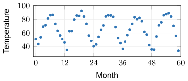
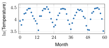
The 60 monthly readings rise and fall once a year for five years. Every peak lands between the low 80s and the low 90s, and every trough between the low 30s and the low 40s. Peak to peak takes about 12 months. The roughly constant extremes and the roughly constant spacing meet the definition of sinusoidal data, and a sine model is reasonable.

The semi-log plot still oscillates and gives no evidence for a different model. R labels its vertical axis log(Temperature), its spelling of $\ln(\text{Temperature})$ .

Example 5

The PollenCountLA dataset, in the MMAC package, records the pollen count in Los Angeles every third day from 1 April 2014, with Date the number of days since 1 April. Determine whether a sine model is reasonable for Count against Date.

ShowHide solution

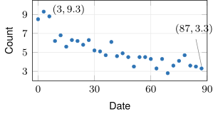
Plot the data with plotPoints(Count ~ Date, data = PollenCountLA).

Pollen follows the seasons, and its expected period is a year. The record covers 87 days, less than a quarter of one period. Over those days the counts drift down, from 9.3 at Date 3 to 3.3 at Date 87, with small rises and falls from one reading to the next at no constant spacing. The plot shows no full cycle and no pair of constant extremes. The data fail the definition of sinusoidal data, and a sine model is not reasonable for this record.

Next: 3. Approximation of the Parameters by Hand Lesson map

3. Approximation of the Parameters by Hand

Objective. Given data exhibiting a sinusoidal relationship, approximate the parameters by hand.

Approximating a sine model by hand.

Choose a level near the top of the data as the maximum $y_{\max}$ , and a level near the bottom as the minimum $y_{\min}$ . Neither has to be exact.
The vertical shift $v$ is the midpoint of the two levels, $v = \frac{y_{\max} + y_{\min}}{2}$ .
The amplitude $A$ is half the distance between the two levels, $A = \frac{y_{\max} - y_{\min}}{2}$ .
The period $P$ is the input distance from one peak to the next, or from one trough to the next.
The horizontal shift $h$ is the first input where the data cross the level $y = v$ while increasing. When the crossing falls between two readings, take the midpoint of their two inputs.
If that shift fails $0 \le h < P$ , then add or subtract whole periods until it satisfies $0 \le h < P$ .

Gridlines. To draw the two axes in heavy black, run mathaxis.on(). To draw light gray gridlines behind the data, run grid.on(col = "lightgrey"). With the grid on, read each level and each input distance against a gridline.

Typical peaks and troughs. A level through the band of typical peaks and one through the band of typical troughs give a better amplitude than the one from the single highest and lowest points. The single highest point may be one unusual reading.

Period from several cycles. With several cycles on the plot, the input distance across all of them divided by the number of cycles gives a steadier period than one peak-to-peak measurement.

Peak to trough. The input distance from a peak to the next trough is half a period. When the plot shows neither two peaks nor two troughs, double the peak-to-trough distance. When the plot lacks a peak or a trough, use the expected period from section 2.

Crossing while increasing. A curve crosses its center line twice per cycle. It is increasing at one crossing and decreasing at the other. An $h$ taken at the crossing while decreasing is off by half a period.

Work shown. Show the two levels in written work, as in $A = \frac{50 - 10}{2}$ , or mark them on the graph.

Example 6

Approximate a sine model for TemperaturesDanville by hand, and plot it on the data.

ShowHide solution

Take 88 as a level near the top of the data and 32 as one near the bottom, the levels MMAC uses, and substitute them into the formulas for the vertical shift and the amplitude:

v = \frac{y_{\max} + y_{\min}}{2} = \frac{88 + 32}{2} = 60, \qquad A = \frac{y_{\max} - y_{\min}}{2} = \frac{88 - 32}{2} = 28.

Peaks land near Month 7, 19, 30, 41, and 55. The 48 months from Month 7 to Month 55 span four cycles, which gives

P = \frac{48}{4} = 12.

The data cross 60 while increasing between Month 2 (53.8) and Month 3 (69.3). The midpoint of the two months gives $h = 2.5$ , which already satisfies $0 \le h < 12$ . The approximate model is

\text{Temperature} = 28\sin\!\left(\frac{2\pi}{12}(\text{Month} - 2.5)\right) + 60.

Plot the model on the data, with gridlines to check the levels:

plotPoints(Temperature ~ Month,
data = TemperaturesDanville)
mathaxis.on()
grid.on(col = "lightgrey")
plotFun(28*sin(2*pi/12*(Month - 2.5))
+ 60 ~ Month, add = TRUE,
col = "magenta2", npts = 10000)

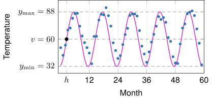
In the figure, the dashed lines are the two levels $y_{\max} = 88$ and $y_{\min} = 32$ and the center line $y = v = 60$ halfway between them. The black point is $(h, v) = (2.5, 60)$ , where the curve crosses the center line while increasing.

The argument npts = 10000 makes R draw the curve through 10000 points in place of the default 500, which can draw the peaks short over a window with many cycles.

Example 7

The TemperaturesDanville data, plotted against the calendar year

\text{Year} = 2006 + \frac{\text{Month}}{12},

first cross their center line while increasing at $\text{Year} = 2006 + \frac{2.5}{12}$ . The period is $P = 1$ year. Give the lowest nonnegative horizontal shift.

ShowHide solution

The crossing lies $2006$ whole periods past $\text{Year} = 0$ , because $\frac{2006 + 2.5/12}{1}$ has whole-number part 2006. Subtracting those 2006 periods gives

h = 2006 + \frac{2.5}{12} - 2006(1) = \frac{2.5}{12} \approx 0.208,

which satisfies $0 \le h < 1$ . In months, the shift is $\frac{2.5}{12} \times 12 = 2.5$ , the crossing at Month 2.5 in the original input.

Next: 4. Best-Fit Sine Model in R Lesson map

4. Best-Fit Sine Model in R

Objective. In R, use fitModel() to obtain the best-fit sine model.

The start = list() argument of fitModel() gives a starting value for each parameter, such as start = list(A = 28, P = 12, h = 2.5, v = 60). The fit searches for the best-fit values beginning from these starting values.

The starting values in the list are the parameters approximated by hand in section 3. After the fit, R’s coef() returns the best-fit $A$ , $P$ , $h$ , and $v$ , ready to substitute into the general form.

Example 8

Find the best-fit sine model for TemperaturesDanville, and draw it on the data.

ShowHide solution

Approximate the starting values by hand as in Example 6, from levels 88 and 32, peaks at Month 7 and Month 55 four cycles apart, and a crossing of 60 while increasing between Month 2 and Month 3:

A = \frac{88 - 32}{2} = 28, \qquad P = \frac{55 - 7}{4} = 12, \qquad h = \frac{2 + 3}{2} = 2.5, \qquad v = \frac{88 + 32}{2} = 60.

Fit the general form to the data from these starting values:

tempModel = fitModel(Temperature ~ A*sin(2*pi/P*(Month - h)) + v,
data = TemperaturesDanville,
start = list(A = 28, P = 12, h = 2.5, v = 60))
coef(tempModel)

The last line prints

A P h v
23.286833 11.982097 3.163625 65.358279

R prints each parameter’s name from the formula above its value. Each number substitutes into the general form for its own letter. The best-fit model is

\text{Temperature} = 23.286833\sin\!\left(\frac{2\pi}{11.982097}(\text{Month} - 3.163625)\right) + 65.358279.

Draw the fitted model function on the data:

plotPoints(Temperature ~ Month,
data = TemperaturesDanville)
plotFun(tempModel(Month) ~ Month,
add = TRUE, col = "red",
npts = 10000)

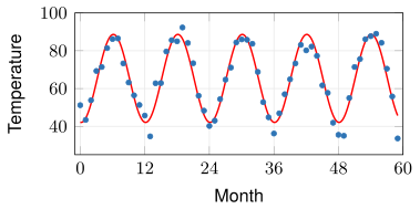
Checking a fitted sine model.

Period check: $P$ is close to the expected period from section 2.
Amplitude check: $A$ is positive and close to half the visible swing of the data.
Shift check: $h$ satisfies $0 \le h < P$ . A fitted $h$ outside that interval gives the same curve, and adding or subtracting whole periods as in section 3 brings it into the interval.
Picture check: the fitted curve, drawn on the data, follows the data.

Example 9

The SunsetGreenwich dataset, in the MMAC package, records the number of minutes after 3 pm until sunset at Greenwich, England, each month since January 2010. Fit a sine model to the data.

ShowHide solution

Approximate the four parameters by hand from a plot, then give them to fitModel() as starting values. Plot the data with gridlines:

plotPoints(Minutes ~ Month,
data = SunsetGreenwich)
mathaxis.on()
grid.on(col = "lightgrey")

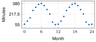
The two Julys in the data, Month 6 and Month 18, peak at 380. The two Decembers, Month 11 and Month 23, bottom out at 55. The two levels give $v$ and $A$ , and the peaks at Month 6 and Month 18 give the period:

v = \frac{380 + 55}{2} = 217.5, \qquad A = \frac{380 - 55}{2} = 162.5, \qquad P = 18 - 6 = 12.

The data cross 217.5 while increasing between Month 2 (160) and Month 3 (273). The midpoint of the two months gives $h = 2.5$ . With these four values as the starting values, fitModel() finds the best-fit sine model:

sunsetModel = fitModel(Minutes ~ A*sin(2*pi/P*(Month - h)) + v,
data = SunsetGreenwich,
start = list(A = 162.5, P = 12, h = 2.5, v = 217.5))
coef(sunsetModel)

The last line prints

A P h v
164.731323 12.013820 2.623386 223.613868

The best-fit model is

\text{Minutes} = 164.731323\sin\!\left(\frac{2\pi}{12.013820}(\text{Month} - 2.623386)\right) + 223.613868.

Common errors.

Missing starting values. A fit without start = stops with an error:
```
> fitModel(Temperature ~ A*sin(2*pi/P*(Month - h)) + v, data = TemperaturesDanville)
Error in nlsModel(formula, mf, start, wts, scaleOffset = scOff, nDcentral = nDcntr) :
  singular gradient matrix at initial parameter estimates
```
With a misspelled name in start = list(), such as H = 2.5 for h, R prints the same singular gradient error. Match the four names in the list to the four parameter names in the formula.
Misplaced parenthesis. With a parenthesis in the wrong place in A*sin(2*pi/P*(Month - h)) + v, R fits a different model and prints no message.
Poor starting period. R never warns that a fit from fitModel() is bad. With a starting period of 5, the fit on TemperaturesDanville comes back with no message:
```
> coef(fitModel(Temperature ~ A*sin(2*pi/P*(Month - h)) + v, data = TemperaturesDanville, start = list(A = 28, P = 5, h = 2.5, v = 60)))
A          P          h          v
-2.052298  4.844543  3.964893 65.377525
```
The negative amplitude fails the amplitude check, and the period of 4.845 months fails the period check.

Next: 5. Evaluation and Interpretation of a Sine Model Lesson map

5. Evaluation and Interpretation of a Sine Model

Objective. Evaluate a sine model at a given input and interpret the answer.

Enter the input to a model function in the dataset’s units. In tempModel(217), the input 217 counts months since January 2006.

Dataset help entry. The help entry ?TemperaturesDanville states what Month counts from and what Temperature is measured in. Values in some datasets are in unusual units, such as minutes after 3 pm or feet above the mean lower water level.

Clock times. Convert a time of day to the dataset’s units. In SunsetGreenwich, which counts minutes after 3 pm, the time 5:30 pm is 150 minutes. In data that count hours after midnight, minutes become a fraction of an hour: 30 minutes is 0.5 hours, and 5:30 pm is 17.5 hours.

Evaluation through the model function. Evaluate a fitted model through its model function, as in tempModel(217), which carries every digit of the four parameters. Rounded parameters retyped by hand move the prediction, and far from the data the change can be much larger than inside it. The call tempModel(217) gives 46.208, while the same four parameters retyped at three decimals give 46.217, and at one decimal 44.114, a change of 2.093 degrees. At Month 30, inside the data, the one-decimal parameters change the output by 0.024 degrees.

Recorded value. The recorded value at an input sits in the dataset’s row with that input value. For example, SunsetGreenwich[SunsetGreenwich$Month == 17, ] prints the row with Month 17. To see the same row in the table, type View(SunsetGreenwich) in the Console.

The recorded value minus the model’s output is the model’s error at that input (Lesson 7 sheet, section 6).

Example 10

The best-fit model of TemperaturesDanville predicts the average maximum temperature in Danville in February 2024. Find the prediction, and state whether it is interpolation or extrapolation.

ShowHide solution

In this dataset, Month 0 is January 2006. January 2024 is Month $(2024 - 2006) \times 12 = 216$ , and February 2024 is Month 217. Starting values come from the data as in Example 6: levels 88 and 32, peaks at Month 7 and Month 55 four cycles apart, and a crossing of 60 while increasing between Month 2 and Month 3:

A = \frac{88 - 32}{2} = 28, \qquad P = \frac{55 - 7}{4} = 12, \qquad h = \frac{2 + 3}{2} = 2.5, \qquad v = \frac{88 + 32}{2} = 60.

Fit the model from these starting values and evaluate it at 217:

tempModel = fitModel(Temperature ~ A*sin(2*pi/P*(Month - h)) + v,
data = TemperaturesDanville,
start = list(A = 28, P = 12, h = 2.5, v = 60))
tempModel(217)

The last line prints [1] 46.20766. The model predicts an average maximum temperature of about 46.208 degrees Fahrenheit in Danville, Kentucky, in February 2024. The prediction is extrapolation (Lesson 4 sheet, section 3), because the data end at Month 59 and Month 217 lies 158 months, about 13 years, past it.

Example 11

Use the best-fit model of SunsetGreenwich to predict the time of sunset at Greenwich in June 2011, and compare the prediction with the recorded value.

ShowHide solution

In this dataset, Month 0 is January 2010, and June 2011 is Month $12 + 5 = 17$ . Starting values come from the data as in Example 9: peaks of 380 at Month 6 and Month 18, troughs of 55, and a crossing of 217.5 while increasing between Month 2 and Month 3:

A = \frac{380 - 55}{2} = 162.5, \qquad P = 18 - 6 = 12, \qquad h = \frac{2 + 3}{2} = 2.5, \qquad v = \frac{380 + 55}{2} = 217.5.

Fit the model from these starting values, evaluate it at 17, and print the recorded row:

sunsetModel = fitModel(Minutes ~ A*sin(2*pi/P*(Month - h)) + v,
data = SunsetGreenwich,
start = list(A = 162.5, P = 12, h = 2.5, v = 217.5))
sunsetModel(17)
SunsetGreenwich[SunsetGreenwich$Month == 17, ]

The call sunsetModel(17) prints [1] 379.1844, in minutes after 3 pm. Splitting off whole hours of 60 minutes gives $379.1844 = 6(60) + 19.1844$ , that is, 6 hours and about 19 minutes after 3 pm. The model predicts sunset at about 9:19 pm in June 2011. The last line prints the recorded row, Minutes 367. Since $367 = 6(60) + 7$ , the recorded sunset is at 9:07 pm, about 12 minutes before the model’s sunset.

Example 12

The best-fit model of TemperaturesDanville has $A = 23.286833$ degrees Fahrenheit. State what $A$ means for Danville’s climate. A model for another city has $A = 19.11$ degrees Fahrenheit. Compare that city’s climate with Danville’s.

ShowHide solution

By the definition of the amplitude, the model’s average maximum temperature in Danville peaks about 23.287 degrees above its center line in summer and bottoms out the same distance below it in winter. The swing from winter to summer is $2A \approx 46.574$ degrees. The other city’s swing is $2(19.11) = 38.22$ degrees, about 8.354 degrees less than Danville’s. That city has milder seasons than Danville.

Lesson map