Lesson 6: Modeling with Exponential Functions II

Objectives

Use a semi-log plot to decide whether an exponential model fits a dataset.
Given data exhibiting an exponential relationship, approximate the parameters by hand.
Determine an appropriate horizontal shift $h$ to use.
In R, use fitModel() to obtain the best-fit exponential model.
Given a semi-log fit $\ln(y) = m(x-h) + b$ , use algebra to write an equivalent model $y = Ce^{k(x-h)}$ or $y = Ce^{kx}$ .
Evaluate an exponential model at a given input and interpret the answer.

1. Semi-Log Test for an Exponential Model

Objective. Use a semi-log plot to decide whether an exponential model fits a dataset.

The semi-log plot of an exponential model with $C > 0$ is a line (Lesson 5 sheet, sections 4 and 5). With a horizontal shift $h$ , the line takes the form below.

Theorem 1 (Shifted exponential model and its semi-log line).

The exponential model $y = Ce^{k(x-h)}$ , with $C > 0$ and horizontal shift $h$ , has the semi-log line

\ln(y) = m(x-h) + b, \qquad m = k, \quad b = \ln(C).

To convert a semi-log line $\ln(y) = m(x-h) + b$ with $m \neq 0$ back to the exponential model, set

k = m, \qquad C = e^{b}.

Semi-log test.

Make the standard plot: plotPoints(y ~ x).
Check that every output $y$ is positive, then make the semi-log plot: plotPoints(log(y) ~ x). Data with an output of zero or less have no semi-log plot.
If the semi-log plot is close to a nonconstant line and straighter than the standard plot, then an exponential model is reasonable.

Judgment call. When both plots are close to a line and neither is straighter, fit the model as in section 4 and check whether its curve follows the data, with the points scattered on both sides of it.

Nonconstant semi-log line. The semi-log test asks for a nonconstant line. A flat semi-log line has slope $k = 0$ . The model $y = Ce^{0(x-h)}$ is then the constant model $y = C$ , which neither grows nor decays.

Example 1

The Mortgage30YrAnnual dataset gives the average 30-year mortgage rate Rate, in percent, for each Year from 1981 to 2012. Determine whether an exponential model is reasonable for Rate as a function of Year.

ShowHide solution

Apply the semi-log test. Plot the data, then plot the logged rates against Year:

plotPoints(Rate ~ Year, data = Mortgage30YrAnnual)
plotPoints(log(Rate) ~ Year, data = Mortgage30YrAnnual)

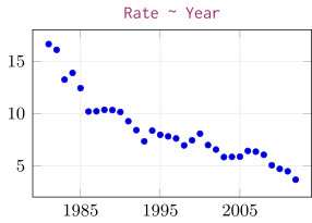
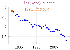
R’s log() is the natural logarithm, and the title log(Rate) ~ Year means the points $(\text{Year}, \ln(\text{Rate}))$ . The 1981 rate, 16.63 percent, plots at height $\ln(16.63) \approx 2.811$ , the orange point. The standard plot drops steeply through the 1980s and flattens after 2000. The semi-log plot falls along a nearly straight line. An exponential model is reasonable, because the semi-log plot is close to a nonconstant line and straighter than the standard plot.

Example 2

The APCalculus dataset gives the number of Advanced Placement Calculus exams taken, Exams, for each Year from 1955 to 2015. Determine whether an exponential model is reasonable for Exams as a function of Year.

ShowHide solution

Plot the data, then plot the logged exam counts against Year:

plotPoints(Exams ~ Year, data = APCalculus)
plotPoints(log(Exams) ~ Year, data = APCalculus)

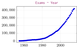
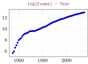
The semi-log plot climbs steeply through the late 1950s and then bends into a much slower rise. An exponential model is not reasonable, because the semi-log plot bends instead of following one line.

Next: 2. Parameters by Hand Lesson map

2. Parameters by Hand

Objective. Given data exhibiting an exponential relationship, approximate the parameters by hand.

A line through the first and last points of the semi-log plot approximates the line that the semi-log points lie close to. As in the textbook, the data are taken in order of increasing input. The first data point has the smallest input, and the last data point has the largest.

Fitting an exponential model by hand.

Set $h$ to the smallest input in the data.
With $(x_{\text{first}}, y_{\text{first}})$ the first data point and $(x_{\text{last}}, y_{\text{last}})$ the last, compute the slope from the logs of the outputs and the inputs as they are:
$m = \frac{\ln(y_{\text{last}}) - \ln(y_{\text{first}})}{x_{\text{last}} - x_{\text{first}}}.$
Set $b = \ln(y_{\text{first}})$ , the value of the semi-log line at $x = h$ , the first data point’s input.
Convert $m$ and $b$ with the shifted exponential model theorem, and write $y = Ce^{k(x-h)}$ .

Example 3

A sealed drum of radioactive material gives off radiation. An instrument at the drum’s surface gives a reading rad, in millirem per hour (mrem/hr), that falls with year, the years since sealing.

`year`	0	2	3.5	6	8
`rad` (mrem/hr)	950	695	538	361	262

Approximate an exponential model for rad as a function of year by hand, from the first and last data points.

ShowHide solution

Because the smallest input is 0, the shift is $h = 0$ and drops out of the model. Substitute the first and last data points, $(0, 950)$ and $(8, 262)$ , into the formulas for the slope and the intercept:

m = \frac{\ln(262) - \ln(950)}{8 - 0} \approx \frac{5.568 - 6.856}{8} = \frac{-1.288}{8} = -0.161, \qquad b = \ln(950).

The slope $m$ is the slope of the dashed line through the first and last semi-log points, $(0, \ln(950))$ and $(8, \ln(262))$ , the filled points in the figure. The intercept $b$ is the height of that line at $\text{year} = h = 0$ . Convert with the shifted exponential model theorem, $k = m$ and $C = e^{b}$ :

k \approx -0.161, \qquad C = e^{\ln(950)} = 950.

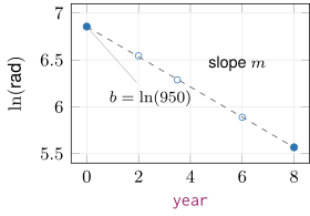
The model is

\text{rad} = 950e^{-0.161\,\text{year}}.

The model gives 950 mrem/hr at sealing, with $k \approx -0.161$ per year.

Example 4

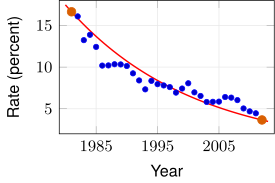
Approximate an exponential model for Rate as a function of Year in Mortgage30YrAnnual by hand, from the first and last data points, $(1981, 16.63)$ and $(2012, 3.66)$ . Plot the model over the data.

ShowHide solution

As in Example 3, with the shift $h = 1981$ , the smallest input, the slope and the intercept are

m = \frac{\ln(3.66) - \ln(16.63)}{2012 - 1981} \approx \frac{1.297 - 2.811}{31} = \frac{-1.514}{31} \approx -0.049, \qquad b = \ln(16.63).

The conversion gives

k \approx -0.049, \qquad C = e^{\ln(16.63)} = 16.63,

and the model is

\text{Rate} = 16.63e^{-0.049(\text{Year} - 1981)}.

In R, store the model at full precision and draw it over the data. The line for m is the slope formula above, and exp(b) is $C = e^{b}$ :

m = (log(3.66) - log(16.63))/(2012 - 1981)
b = log(16.63)
f = makeFun(exp(b)*exp(m*(Year - 1981)) ~ Year)
plotPoints(Rate ~ Year, data = Mortgage30YrAnnual)
plotFun(f(Year) ~ Year, add = TRUE, col = "red")

The red curve passes through the first and last data points, $(1981, 16.63)$ and $(2012, 3.66)$ , the orange points, because the hand fit is built from those two points alone. The 30 rates in between fall on both sides of the curve: 14 lie above it and 16 below it.

Next: 3. Horizontal Shift Lesson map

3. Horizontal Shift

Objective. Determine an appropriate horizontal shift $h$ to use.

Shift from the smallest input. The horizontal shift $h$ of $y = Ce^{k(x-h)}$ (Lesson 5 sheet, section 2) is set to the smallest input in the data. It comes from the data and is never estimated.

With this shift, $C$ is the model’s value at the first data point’s input, because $y = Ce^{k(x-h)}$ equals $C$ at $x = h$ . Without the shift, the constant in front of the exponential is the model’s value at $x = 0$ . That input can lie far outside the data.

Unshifted mortgage model. Writing Example 4’s semi-log line without the shift moves the intercept to Year 0:

\ln(\text{Rate}) = m(\text{Year} - 1981) + b = m\,\text{Year} + (b - 1981m).

With $m = -0.04883049$ , the slope Example 4 stores in R at full precision (typing m prints [1] -0.04883049), and $b = \ln(16.63)$ , the new intercept is

b - 1981m \approx 99.544,

and the model is

\text{Rate} = e^{b - 1981m}e^{m\,\text{Year}} \approx (1.704 \times 10^{43})\,e^{-0.049\,\text{Year}}.

Both forms describe the same model when $m$ and $b$ keep full precision. The rounded slope $-0.049$ gives about 11.9 at 1981 in place of 16.63. Compute outputs of the unshifted form from the stored $m$ and $b$ .

The unshifted constant $1.704 \times 10^{43}$ is the model’s rate for Year 0, 1981 years before the data begin, and has no meaning for mortgage rates. The shifted form is used because its constant, $C = 16.63$ , is a rate inside the data: the rate in 1981, the first year recorded.

Example 5

The table gives six rows of the NetherlandsPopulation dataset: the population of the Netherlands, in millions, every 20 years from 1850 to 1950.

`Year`	1850	1870	1890	1910	1930	1950
`Population`	3.0840	3.5950	4.5150	5.8582	7.8250	10.0268

Determine the horizontal shift $h$ for an exponential model of Population as a function of Year fitted to these six rows.

ShowHide solution

The shift is the smallest value of the input Year, $h = 1850$ , and the model has the form

\text{Population} = Ce^{k(\text{Year} - 1850)}.

With this shift, $C$ is the model’s population in 1850, the first year in the data.

Example 6

The table gives air pressure, in inches of mercury, at altitudes in thousands of feet.

Altitude	0	5	10	15	20	25	30
Pressure	29.92	24.90	20.58	16.89	13.75	11.10	8.89

Determine the horizontal shift $h$ for an exponential model of Pressure as a function of Altitude, and state what $C$ means for that model.

ShowHide solution

The shift is the smallest value of the input Altitude, $h = 0$ , which drops out of the model:

\text{Pressure} = Ce^{k(\text{Altitude} - 0)} = Ce^{k\,\text{Altitude}}.

The constant $C$ is the model’s pressure in inches of mercury at sea level, altitude 0. That altitude is the first one in the data.

Next: 4. Best-Fit Exponential Model in R Lesson map

4. Best-Fit Exponential Model in R

Objective. In R, use fitModel() to obtain the best-fit exponential model.

For an exponential model, the command fitModel() (Lesson 4 sheet, section 3) fits the shifted semi-log line to every semi-log point. The method of section 2 uses only the first and last.

fitModel() for an exponential model.

bfit = fitModel(log(y) ~ m*(x - h) + b, data = D)
coef(bfit)

In this command, y, x, and D are the output, the input, and the dataset. Type the shift $h$ in as a number. R estimates $m$ and $b$ , and coef() prints them. For data typed in with c(), as in Example 8, leave off data = D.

The fitted model function is the R function that fitModel() returns. Given an input $x$ , it returns the fitted model’s output $y$ , including when the formula is fitted to log(y). In the command above, the fitted model function is bfit.

[2]

Example 7

Find the best-fit exponential model for Rate as a function of Year in Mortgage30YrAnnual, and plot it over the data.

ShowHide solution

The shift is $h = 1981$ , the smallest Year. Fit the semi-log line in the shifted form and print its slope and intercept:

bfit = fitModel(log(Rate) ~ m*(Year - 1981) + b, data = Mortgage30YrAnnual)
coef(bfit)

The last line prints

m b
-0.03739385 2.64752113

R labels each estimate with its name in the formula: m is the slope and b the intercept of the semi-log line. Convert with $k = m$ and $C = e^{b}$ :

k \approx -0.037, \qquad C = e^{2.64752113} \approx 14.119,

and the model is

\text{Rate} = 14.119e^{-0.037(\text{Year} - 1981)}.

Plot the fitted model function over the data:

=1.5em plotPoints(Rate ~ Year,
data = Mortgage30YrAnnual)
plotFun(bfit(Year) ~ Year,
add = TRUE, col = "red")

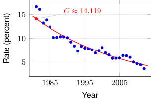
The red curve starts at $C \approx 14.119$ in 1981, the shift $h$ . The curve follows the fall of the data: 15 of the 32 recorded rates lie above it and 17 below it, and the largest gap is 2.511 percentage points, in 1981.

Example 8

The table gives six rows of the NetherlandsPopulation dataset: the population of the Netherlands, in millions, every 20 years from 1850 to 1950.

`Year`	1850	1870	1890	1910	1930	1950
`Population`	3.0840	3.5950	4.5150	5.8582	7.8250	10.0268

Type the six rows into R as vectors, and find the best-fit exponential model for Population as a function of Year.

ShowHide solution

The shift is $h = 1850$ , the smallest Year. Type in the data and fit as in Example 7:

Year = c(1850, 1870, 1890, 1910, 1930, 1950)
Population = c(3.0840, 3.5950, 4.5150, 5.8582, 7.8250, 10.0268)
pfit = fitModel(log(Population) ~ m*(Year - 1850) + b)
coef(pfit)

The last line prints

m b
0.01212707 1.06758071

Then

k \approx 0.012, \qquad C = e^{1.06758071} \approx 2.908,

and the model is

\text{Population} = 2.908e^{0.012(\text{Year} - 1850)}.

Fitted model over a semi-log plot. Draw the log of the model’s output over a semi-log plot:

bfit = fitModel(log(Rate) ~ m*(Year - 1981) + b, data = Mortgage30YrAnnual)
plotPoints(log(Rate) ~ Year, data = Mortgage30YrAnnual)
plotFun(log(bfit(Year)) ~ Year, add = TRUE, col = "red")

Without the log, plotFun(bfit(Year) ~ Year, add = TRUE) draws nothing and prints no error, because the curve lies entirely above the window of the semi-log plot. The model’s rates run from 14.119 down to about 4.4, and the vertical axis of the semi-log plot stops near 2.8.

Errors in the shifted formula. When the * between m and the parentheses is missing, R reports a function m that does not exist:

> bfit = fitModel(log(Rate) ~ m(Year - 1981) + b, data = Mortgage30YrAnnual)
Error in m(Year - 1981) : could not find function "m"

A fitModel() command typed without the parentheses, as m*Year - 1981 + b, runs with no error and fits an unshifted line: coef() prints $b \approx 2057.725$ in place of 2.648.

Next: 5. Equivalent Exponential Models Lesson map

5. Equivalent Exponential Models

Objective. Given a semi-log fit $\ln(y) = m(x-h) + b$ , use algebra to write an equivalent model $y = Ce^{k(x-h)}$ or $y = Ce^{kx}$ .

Exponentiating both sides of the semi-log line undoes the log, because $e^{\ln(y)} = y$ :

y = e^{m(x-h) + b} = e^{b}e^{m(x-h)}.

Naming $C = e^{b}$ and $k = m$ gives $y = Ce^{k(x-h)}$ .

Unshifted form. Splitting the exponent once more removes the shift:

Ce^{k(x-h)} = Ce^{-kh}e^{kx}.

The unshifted constant is $Ce^{-kh}$ .

Example 9

A dataset has the semi-log line

\ln(y) = 0.0518(x - 12) + 1.427.

Write the equivalent exponential model.

ShowHide solution

The conversions $k = m$ and $C = e^{b}$ give

k = 0.0518, \qquad C = e^{1.427} \approx 4.166.

The model is

y = 4.166e^{0.0518(x - 12)}.

Example 10

Write the semi-log line of the exponential model

y = 250e^{-0.12(x - 3)}.

ShowHide solution

The conversions $m = k$ and $b = \ln(C)$ give

m = -0.12, \qquad b = \ln(250) \approx 5.521.

The semi-log line is

\ln(y) = -0.12(x - 3) + 5.521.

Example 11

Write the best-fit mortgage model of Example 7,

\text{Rate} = 14.119e^{-0.037(\text{Year} - 1981)},

in the unshifted form $\text{Rate} = Ae^{k\,\text{Year}}$ .

ShowHide solution

The unshifted constant is $A = Ce^{-kh}$ with $h = 1981$ . R computes it from coef(bfit) at full precision:

bfit = fitModel(log(Rate) ~ m*(Year - 1981) + b, data = Mortgage30YrAnnual)
cf = coef(bfit)
exp(cf["b"])*exp(-cf["m"]*1981)

The last line prints 2.094724e+33, under the label b. The model is

\text{Rate} \approx (2.095 \times 10^{33})\,e^{-0.037\,\text{Year}}.

Outputs come from the fitted model function bfit, which keeps $k$ and $C$ at full precision. At 1981, this rounded form gives about 30.811 in place of 14.119,

(2.095 \times 10^{33})\,e^{-0.037(1981)} \approx 30.811.

Early rounding. Rounding $k$ to $-0.037$ first gives

14.119e^{0.037(1981)} \approx 9.600 \times 10^{32}.

That constant is less than half the full-precision value. The rounding error in $k$ is multiplied by 1981 inside the exponent.

Next: 6. Predictions and Interpretation Lesson map

6. Predictions and Interpretation

Objective. Evaluate an exponential model at a given input and interpret the answer.

To evaluate the model at full precision, give the input to the fitted model function: bfit(2015) returns the model’s output for Year 2015. Each prediction is an interpolation or an extrapolation (Lesson 4 sheet, section 3).

Prediction and recorded value. The model’s output is a prediction. The dataset records the value that occurred. State the model’s output as a prediction, with units, and keep it separate from the recorded value.

Example 12

Use the best-fit exponential model for Mortgage30YrAnnual to predict the average 30-year mortgage rate in 2015, in mid-1993, and in 1884. Interpret each answer.

ShowHide solution

Evaluate the fitted model function at each year:

bfit = fitModel(log(Rate) ~ m*(Year - 1981) + b, data = Mortgage30YrAnnual)
bfit(2015)
bfit(1993.5)
bfit(1884)

The last three lines print [1] 3.95955, [1] 8.847174, and [1] 530.9799.

The model predicts an average rate of 3.960 percent in 2015. The prediction is an extrapolation, because the data stop at 2012.
The model predicts an average rate of 8.847 percent in mid-1993. The prediction is an interpolation, because 1993.5 lies inside the data’s years, 1981 to 2012.
The model predicts an average rate of 530.980 percent in 1884. The prediction is an extrapolation, because 1884 lies 97 years before the data begin. The model gives no usable rate that far outside the data, because 530.980 percent is more than 30 times the largest recorded rate, 16.63 percent.

Example 13

Compare the best-fit mortgage model’s output for 2000 with the rate recorded in Mortgage30YrAnnual for 2000.

ShowHide solution

Evaluate the fitted model function at 2000:

bfit = fitModel(log(Rate) ~ m*(Year - 1981) + b, data = Mortgage30YrAnnual)
bfit(2000)

The last line prints [1] 6.93817. The model predicts an average rate of 6.938 percent in 2000. To find the recorded rate, type View(Mortgage30YrAnnual) in the Console. The row for Year 2000 records a rate of 8.06 percent, about 1.122 percentage points above the prediction.

Example 14

`year`	0	2	3.5	6	8
`rad` (mrem/hr)	950	695	538	361	262

Use the best-fit exponential model to predict the reading 10 years after sealing, and interpret the answer.

ShowHide solution

Because the smallest input is 0, the shift is $h = 0$ and drops out of the formula given to fitModel(). Type in the data, fit as in Example 8, and evaluate the fitted model function at 10:

year = c(0, 2, 3.5, 6, 8)
rad = c(950, 695, 538, 361, 262)
rfit = fitModel(log(rad) ~ m*year + b)
rfit(10)

The last line prints [1] 189.426. The model predicts a reading of 189.426 mrem/hr 10 years after sealing. By the model, the drum can be shipped at 10 years, because the predicted reading is below the 200 mrem/hr limit. The prediction is an extrapolation beyond the last reading at 8 years.

Lesson map