Existence of Linear Combinations
Looking ahead
Objectives
- Use errors returned by
solve()to determine whether a unique solution exists. - Given a vector equation, use R to determine whether a satisfying linear combination exists.
- Given data, write a vector equation representing a linear model that fits perfectly; determine whether it has a solution and what that says about the dataset.
1. Errors from solve()
Objective. Use errors returned by solve() to determine whether a unique solution exists.
Theorem 1 (Number of solutions).
A system of linear equations has exactly one solution, no solution, or infinitely many solutions.
Definition 2 (Unique solution).
A system of linear equations has a unique solution when it has exactly one solution.
The system of the equations and has no unique solution, because both and solve both equations. The definition requires exactly one solution.
With two unknowns, the graph of each equation is a line, and the three cases match the three ways two lines can lie in the plane. In each graph below, and count two kinds of containers on a pallet. One equation matches the load’s weight in pounds, and the other matches its volume in cubic feet. A case of Meals, Ready-to-Eat (MRE) weighs 22 lb and takes 1 ft, a water can weighs 45 lb and takes 0.9 ft, and a double MRE case weighs 44 lb and takes 2 ft. The first load is MRE cases and water cans, and the second and third are MRE cases and double MRE cases. The first two loads weigh 2230 lb, the third weighs 1474 lb, and each takes 67 ft.
Exactly one solution
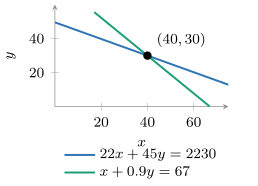
With MRE cases and water cans, the lines cross at : the load is 40 MRE cases and 30 water cans.
No solution
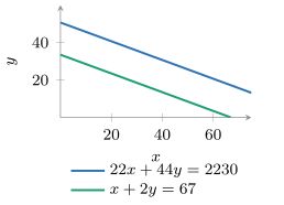
With double MRE cases, the lines are parallel: no load weighs 2230 lb and takes 67 ft.
Infinitely many solutions
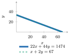
With a 1474 lb load, the lines coincide: every point on the line solves both equations, and every whole-number load with has that weight and volume.
The command solve(A, v) (Lesson 18 sheet, section 4) returns the unknowns only when exactly one solution exists. In the other two cases solve() stops with an error. Because the error depends on the matrix alone, solve() prints the same message for a system with no solution and for a system with infinitely many solutions when the two share a matrix.
Example 1
Use solve() to determine whether each system has a unique solution:
ShowHide solution
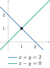
(a) The lines cross at .
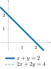
(b) The lines are the same line.
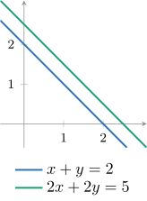
(c) The lines are parallel.
Solve system (a) in R, with the coefficients of as column 1 of the matrix and the coefficients of as column 2:
u1 = c(1, 1)
u2 = c(1, -1)
A = matrix(c(u1, u2), nrow = 2, ncol = 2)
v = c(2, 0)
solve(A, v)
The last line prints [1] 1 1: system (a) has a unique solution, and . Systems (b) and (c) share a matrix. Define it once, and run solve() with each target vector:
u1 = c(1, 2)
u2 = c(1, 2)
A = matrix(c(u1, u2), nrow = 2, ncol = 2)
v = c(2, 4)
solve(A, v)
v = c(2, 5)
solve(A, v)
Both calls print the same error:
Error in solve.default(A, v) :
Lapack routine dgesv: system is exactly singular: U[2,2] = 0
Neither (b) nor (c) has a unique solution, because solve() stops with an error for each. System (b) has infinitely many solutions, because its second equation is twice the first and both equations describe one line. System (c) has no solution, because dividing its second equation by 2 gives , which contradicts .
Messages from solve().
- Numbers, such as
[1] 1 1
Exactly one solution exists. Lapack routine dgesv: system is exactly singular: U[2,2] = 0
No unique solution exists. The system has no solution or infinitely many solutions.system is computationally singular: reciprocal condition number = 1.15648e-17
R stops without a solution. Because decimal entries carry tiny rounding errors, R can find a number near 0 where exact arithmetic gives 0, and then no unique solution exists. The same message can also appear for a system with exactly one solution when one column is very nearly a linear combination of the others. Writing one equation per component and solving the equations by hand settles which case applies.'a' (5 x 2) must be square
R stops with an error, because the matrix is not square. Nothing about the number of solutions follows from this message.
Example 2
Use solve() to determine whether the matrix equation has a unique solution:
ShowHide solution
Define the three columns, the matrix, and the target vector, then run solve():
u1 = c(0.1, 0.2, 0.3)
u2 = c(0.4, 0.5, 0.6)
u3 = c(0.7, 0.8, 0.9)
A = matrix(c(u1, u2, u3), nrow = 3, ncol = 3)
v = c(0.5, 0.7, 0.9)
solve(A, v)
The last line prints
Error in solve.default(A, v) :
system is computationally singular: reciprocal condition number = 5.78241e-18
After a computationally singular message, the number of solutions is still open, and a check of the columns by hand settles it. The columns step by the same amount: every entry of is 0.3 more than the corresponding entry of , and every entry of is 0.3 more than the corresponding entry of . Column 3 is therefore a linear combination of columns 1 and 2:
Two different sets of scalars then give the target vector. The first adds columns 1 and 2:
The second replaces by :
the same combination as the first set. R computes both linear combinations:
1*u1 + 1*u2 + 0*u3
0*u1 + 3*u2 - 1*u3
Both lines print [1] 0.5 0.7 0.9. The matrix equation has more than one solution, and therefore no unique solution exists.
Singular errors in the textbook. Ch 3.3 of the textbook (page 300) explains that a singular error means no solution or infinitely many solutions, and states that the book’s exercises are set up so that the error always means no solution. Exercise 45 of Ch 3.3, which is Example 4 below, is one exception: it gives a singular error and has infinitely many solutions.
Next: 2. Existence of a Linear CombinationLesson map
2. Existence of a Linear Combination
Objective. Given a vector equation, use R to determine whether a satisfying linear combination exists.
Asking whether is a linear combination of and is asking whether the vector equation
has a solution. With and as the columns of , the vector equation becomes the matrix equation , with the vector of unknowns . When is square, the command solve(A, v) returns the scalars when exactly one set exists.
Existence of a linear combination.
- Make the vectors the columns of , and run
solve(A, v). - If R prints numbers, is a linear combination in exactly one way.
- If R prints a singular error, or is not square, write one equation per component and solve the equations by hand.
- If the equations contradict each other, is not a linear combination. If a scalar can take every value and the others follow from it, is a linear combination in infinitely many ways.
Numerical output. When solve(A, v) prints numbers, the vector is a linear combination of and in exactly one way, with the printed numbers as the scalars. A printout of [1] 1 2, for example, means that .
Singular error. When solve(A, v) prints an exactly singular error, no unique set of scalars exists, because and lie on one line through the origin. Solving the equations by hand then separates the two cases, as the vectors and show. In each graph the dashed line is the line through the origin that contains every linear combination of and .
Target vector on the line
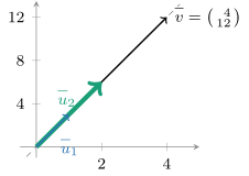
The vector lies on the line. The component equations of are and , and the second is three times the first. For every value of , the scalars and solve both equations. The vector is therefore a linear combination in infinitely many ways.
Target vector off the line
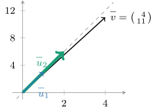
The vector lies off the line. Three times the first component equation, , gives , which contradicts the second equation, . The vector is therefore not a linear combination of and .
Example 3
Determine whether is a linear combination of and :
ShowHide solution
By the definition of a linear combination (Lesson 17 sheet), is a linear combination of and when scalars and give . Solve the matrix equation in R, with and as the columns of :
u1 = c(1, 2)
u2 = c(3, 1)
v = c(7, 4)
A = matrix(c(u1, u2), nrow = 2, ncol = 2)
solve(A, v)
The last line prints [1] 1 2, the only scalars that solve the vector equation. By hand, the two components of are the equations
Solve the second equation for and substitute it into the first:
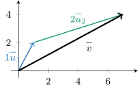
Substituting into gives , the same scalars R found. The vector is a linear combination of and , with . In the figure, runs from the origin, and starts at its tip and ends at .
Example 4
Determine whether is a linear combination of , , and :
ShowHide solution
Solve the matrix equation in R as in Example 3, with the three vectors as the columns of :
u1 = c(5, 3, 1)
u2 = c(4, 1, 0)
u3 = c(8, 2, 0)
v = c(0.5, 0.3, 0.1)
A = matrix(c(u1, u2, u3), nrow = 3, ncol = 3)
solve(A, v)
The last line prints
Error in solve.default(A, v) :
Lapack routine dgesv: system is exactly singular: U[3,3] = 0
No unique set of scalars exists, because solve() prints an exactly singular error. By hand, the three components of are the equations
Substitute , from the third equation, into the first two:
Both reduce to . For every value of , the scalars , , and solve all three equations. As a check, the sets for and give the target vector in R:
u1 = c(5, 3, 1)
u2 = c(4, 1, 0)
u3 = c(8, 2, 0)
0.1*u1 + 0*u2 + 0*u3
0.1*u1 - 2*u2 + 1*u3
Both lines print [1] 0.5 0.3 0.1. The vector is a linear combination of , , and in infinitely many ways, for example .
Example 5
Determine whether is a linear combination of , , and :
ShowHide solution
Solve the matrix equation in R as in Example 4:
u1 = c(0, 1, 2)
u2 = c(1, 1, 0)
u3 = c(2, 2, 0)
v = c(2, 3, 1)
A = matrix(c(u1, u2, u3), nrow = 3, ncol = 3)
solve(A, v)
The last line prints
Error in solve.default(A, v) :
Lapack routine dgesv: system is exactly singular: U[3,3] = 0
No unique set of scalars exists, because solve() prints an exactly singular error. By hand, the three components give the equations
The third equation gives . Substitute it into the second:
which contradicts the first equation, . The vector is not a linear combination of , , and .
Columns behind a singular error. An exactly singular error means one column of is a linear combination of the other columns. In each of Examples 4 and 5, every linear combination of the three columns lies in a single plane, because and neither of and is a scalar multiple of the other. Example 4’s target vector lies in its plane and is a linear combination of the columns. Example 5’s target vector lies off its plane and is not.
Next: 3. Vector Equations for a Perfect FitLesson map
3. Vector Equations for a Perfect Fit
Objective. Given data, write a vector equation representing a linear model that fits perfectly; determine whether it has a solution and what that says about the dataset.
Definition 3 (Perfect fit).
A linear model fits a dataset perfectly when every data point satisfies it.
The model does not fit the data points , , and perfectly. The first two points satisfy it, and the point does not, because . The definition requires every data point to satisfy the model.
For a dataset of data points, each data point , for , gives one equation .
The intercept vector is the vector whose components are all 1.
Stacking the equations gives one vector equation:
In the vector equation of a linear model, the outputs form the target vector, the inputs form the input vector that multiplies, and is the scalar that multiplies the intercept vector.
When , the matrix equation for this vector equation has a matrix with rows and two columns. A matrix that is not square makes solve() stop with an error. When , the matrix is , and solve() returns and when the two -values differ. Two data points with the same -value lie on a vertical line, which has no slope , and solve() prints a singular error.
Existence of a perfect fit.
- Choose two data points with different -values and find the and of the line through them, by the slope formula or with
solve()on the matrix equation for those two points. - Compute times the input vector plus .
- Compare the result with the target vector, component by component. If every component matches, and solve the vector equation. If one or more components differ, the vector equation has no solution.
Mismatched component. Every solution of the vector equation satisfies the two component equations for the data points chosen to find and . Because their -values differ, those two equations have exactly one solution, the and of the line through the two points. As a result, when that line misses another data point, the vector equation has no solution.
Verdict about the data. Data are exactly linear when every data point lies on one line. For data with at least two different -values, a solution of the vector equation means the data are exactly linear, and no solution means the data are not exactly linear. A linear model can still be reasonable for data that are not exactly linear.
Graphical check. Plot the data with plotPoints() and the line through the two chosen points with plotFun(..., add = TRUE). The plot shows whether the line passes through every data point.
Example 6
The table gives the number of Twitter users, in millions, by quarter, where Year counts years since 2000 and is January to March 2011.
| Year | 11 | 11.25 | 11.5 | 11.75 | 12.75 |
| Users (millions) | 68 | 85 | 101 | 117 | 185 |
- (a)
Write the vector equation for a perfect fit of the linear model
- (b) Find and from the first two data points.
- (c) Determine algebraically whether and solve the vector equation, and state the conclusion about the data.
- (d) Show the answer to part (c) graphically.
ShowHide solution
(a) Writing one equation per data point and stacking the five equations gives the vector equation
(b) Substitute the first two data points, and , into the slope formula. Then substitute and the first data point, and , into , and solve for :
In R, solve the matrix equation formed by the first two components:
u1 = c(11, 11.25)
u2 = c(1, 1)
A = matrix(c(u1, u2), nrow = 2, ncol = 2)
solve(A, c(68, 85))
The last line prints [1] 68 -680: and .
(c) By the definition of a perfect fit, the model fits only when every data point satisfies it, that is, when and solve the vector equation. Substituting and into the right side gives
R computes the same right side from the vectors Year and Users:
Year = c(11, 11.25, 11.5, 11.75, 12.75)
Users = c(68, 85, 101, 117, 185)
68*Year - 680
The last line prints [1] 68 85 102 119 187. The first two components match the target vector, and the third is 102 where the target vector has 101. The vector equation has no solution, because the third component differs, and therefore the Twitter data are not exactly linear.
(d) Plotting the data with the line through the first two points shows the answer to part (c):
=2.2em Year = c(11, 11.25, 11.5, 11.75, 12.75)
Users = c(68, 85, 101, 117, 185)
plotPoints(Users ~ Year)
f = makeFun(68*x - 680 ~ x)
plotFun(f(x) ~ x, add = TRUE, col = "red")
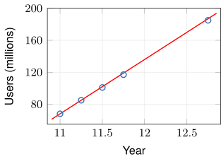
The line passes through the first two points and runs above each of the last three, by 1, 2, and 2 million users. Gaps that small are hard to see against an axis that spans more than 100 million users. Zooming the plot in on the last three points shows each one below the line, the graphical sign that the data are not exactly linear.
Example 7
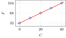
The table lists five temperatures, each in degrees Celsius and in degrees Fahrenheit .
| Celsius | 0 | 10 | 20 | 30 | 40 |
| Fahrenheit | 32 | 50 | 68 | 86 | 104 |
Write the vector equation for a perfect fit of the linear model
Then find and from the first and last data points, determine whether they solve the vector equation, and state the conclusion about the data.
ShowHide solution
Writing one equation per data point gives the vector equation
The line through and has slope and intercept
because the first data point has . Substituting and into the right side gives
Every component matches the target vector. R computes the same right side from the vectors Celsius and Fahrenheit:
Celsius = c(0, 10, 20, 30, 40)
Fahrenheit = c(32, 50, 68, 86, 104)
1.8*Celsius + 32
The last line prints [1] 32 50 68 86 104. The values and solve the vector equation. The data are exactly linear, on the line , because every data point satisfies the model. Each column of the table is one plotted point, such as , and every point lies on the line.