Application to Data
Looking ahead
Objectives
- Apply skills learned in Block 1 to data.
Plutonium Record
The table lists yield readings for a bare plutonium sphere by neutron generation. The source is Bridgman, Introduction to the Physics of Nuclear Weapons Effects, Table 2-10. The input generation counts cycles of neutron multiplication. The output yield_KT is the energy released so far, in kilotons (KT).
| First 24 readings | Ten later readings | ||||
| generation | yield (KT) | generation | yield (KT) | generation | yield (KT) |
| 1 | 40 | 52 | 7.92 | ||
| 5 | 41 | 53 | 11.50 | ||
| 10 | 42 | 54 | 14.70 | ||
| 15 | 43 | 0.0132 | 55 | 17.00 | |
| 20 | 44 | 0.0298 | 56 | 18.50 | |
| 25 | 45 | 0.0668 | 57 | 19.40 | |
| 30 | 46 | 0.148 | 58 | 19.90 | |
| 35 | 47 | 0.323 | 59 | 20.10 | |
| 36 | 48 | 0.685 | 60 | 20.20 | |
| 37 | 49 | 1.40 | 61 | 20.30 | |
| 38 | 50 | 2.71 | |||
| 39 | 51 | 4.87 | |||
1. Applying Block 1 to Data
Objective. Apply skills learned in Block 1 to data.
Example 1
Model the first 24 readings.
- (a) Determine the model family that fits the readings.
- (b) Estimate the parameters by hand from the first and last readings.
- (c) Use
fitModel()to find the best-fit model. - (d) Plot the fitted model over the readings.
ShowHide solution
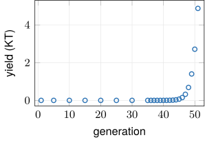
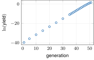
(a) Plot the first 24 readings on a standard plot and on a semi-log plot, as the semi-log test of the Lesson 6 sheet, section 1, requires.
generation = c(1, 5, 10, 15, 20, 25, 30, 35,
36, 37, 38, 39, 40, 41, 42, 43,
44, 45, 46, 47, 48, 49, 50, 51)
yield_KT = c(6.66e-18, 3.12e-16, 1.93e-14, 1.19e-12,
7.32e-11, 4.54e-9, 2.83e-7, 1.78e-5, 4.07e-5,
9.31e-5, 2.13e-4, 4.88e-4, 1.11e-3, 2.55e-3,
5.80e-3, 0.0132, 0.0298, 0.0668, 0.148, 0.323,
0.685, 1.40, 2.71, 4.87)
plotPoints(yield_KT ~ generation)
plotPoints(log(yield_KT) ~ generation)
Each generation and yield pair in the first 24 readings is one point on each plot: the reading 4.87 at generation 51 is the highest point on the standard plot and the point on the semi-log plot. R spells as log(yield_KT), because log() in R is the natural logarithm.
The standard plot is not linear, because the readings sit near 0 through generation 45 and rise steeply after it. The semi-log plot is close to linear from generation 5 to generation 44, because the slopes between consecutive points there all lie between 0.814 and 0.832. Between generations 5 and 10, for example, the semi-log slope is
The readings through generation 44 therefore suit an exponential model:
The semi-log plot bends down over the last readings, where the slope between generations 50 and 51 falls to
Those last readings grow more slowly than the exponential model. Example 3 follows that slowdown into the later readings.
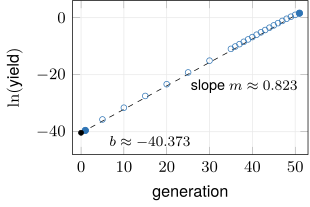
(b) The semi-log form of the exponential model is , with and , as derived on the Lesson 5 sheet, section 4. The two points are the first and last readings on the semi-log plot, and . Substitute them into the slope formula of the two-point method (Lesson 6 sheet, section 2):
Here the model keeps no horizontal shift, so that its compares directly with the fitted of part (c). Solve for the intercept , the height of the line at generation 0, from the first point:
Convert and to the exponential parameters:
In the figure, the filled points are the first and last readings. The dashed line through them has slope , and its height at generation 0 is .
Compute the same parameters in R, with every value stored at full precision:
y1 = log(6.66e-18)
y2 = log(4.87)
m = (y2 - y1)/(51 - 1)
b = y1 - m*1
k = m
C = exp(b)
k
C
R returns and , the hand values at full precision.
(c) Fit the semi-log line to the two vectors from part (a), then convert its slope and intercept to and by the method of the Lesson 6 sheet, sections 4 and 5:
bomb_ln = fitModel(log(yield_KT) ~ m*generation + b)
coef(bomb_ln)
cf = coef(bomb_ln)
k = cf[1]
C = exp(cf[2])
C
R returns the slope , the intercept , and . The output of coef() names each number by its letter in the formula, so cf[1] is the slope and cf[2] is the intercept .
The fitted intercept is above the hand intercept of part (b), because fitModel() uses all 24 readings and the hand line uses two. The fitted is therefore about times the hand value. The best-fit model is
(d) Define the model from the stored and and draw it over the first 24 readings:
=2.2em bomb = makeFun(C*exp(k*generation) ~
generation)
plotPoints(yield_KT ~ generation)
plotFun(bomb(generation) ~ generation,
add = TRUE, col = "purple")
bomb(51)
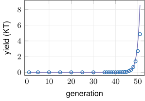
The purple curve is the model, drawn with col = "purple". It stays within 0.01 kilotons of every reading through generation 47 and then rises above the readings. The last line returns kilotons at generation 51, against the reading of 4.87.
Example 2
Use the exponential model of Example 1 to predict the yield at generation 61, and classify the prediction as an interpolation or an extrapolation.
ShowHide solution
Rebuild the model of Example 1 and evaluate it at generation 61:
generation = c(1, 5, 10, 15, 20, 25, 30, 35,
36, 37, 38, 39, 40, 41, 42, 43,
44, 45, 46, 47, 48, 49, 50, 51)
yield_KT = c(6.66e-18, 3.12e-16, 1.93e-14, 1.19e-12,
7.32e-11, 4.54e-9, 2.83e-7, 1.78e-5, 4.07e-5,
9.31e-5, 2.13e-4, 4.88e-4, 1.11e-3, 2.55e-3,
5.80e-3, 0.0132, 0.0298, 0.0668, 0.148, 0.323,
0.685, 1.40, 2.71, 4.87)
bomb_ln = fitModel(log(yield_KT) ~ m*generation + b)
cf = coef(bomb_ln)
k = cf[1]
C = exp(cf[2])
bomb = makeFun(C*exp(k*generation) ~ generation)
bomb(61)
R returns a predicted yield of 32,659.54 kilotons at generation 61. The prediction is an extrapolation as defined on the Lesson 10 sheet, section 6, because generation 61 lies outside the inputs of the first 24 readings, generation 1 to 51.
Example 3
The ten later readings run from generation 52 to generation 61. Compare the exponential model of Example 1 with four of them, at generations 52, 55, 58, and 61. State whether the model fits the ten later readings.
ShowHide solution
Rebuild the model of Example 1 and evaluate it at the four generations:
generation = c(1, 5, 10, 15, 20, 25, 30, 35,
36, 37, 38, 39, 40, 41, 42, 43,
44, 45, 46, 47, 48, 49, 50, 51)
yield_KT = c(6.66e-18, 3.12e-16, 1.93e-14, 1.19e-12,
7.32e-11, 4.54e-9, 2.83e-7, 1.78e-5, 4.07e-5,
9.31e-5, 2.13e-4, 4.88e-4, 1.11e-3, 2.55e-3,
5.80e-3, 0.0132, 0.0298, 0.0668, 0.148, 0.323,
0.685, 1.40, 2.71, 4.87)
bomb_ln = fitModel(log(yield_KT) ~ m*generation + b)
cf = coef(bomb_ln)
k = cf[1]
C = exp(cf[2])
bomb = makeFun(C*exp(k*generation) ~ generation)
bomb(c(52, 55, 58, 61))
R returns the four model values in the second column of the table, and the third column gives the readings from the Plutonium Record:
| generation | model (KT) | reading (KT) | model reading |
| 52 | 19.62 | 7.92 | 2.5 |
| 55 | 232.51 | 17.00 | 13.7 |
| 58 | 2,755.64 | 19.90 | 138.5 |
| 61 | 32,659.54 | 20.30 | 1,608.8 |
The exponential model does not fit the ten later readings. It is 2.5 times the reading at generation 52 and 1,608.8 times the reading at generation 61, because the later readings level off near 20 kilotons and the model grows without bound. The readings level off because the sphere expands until it is no longer critical and the chain reaction stops.
Example 4
Model all 34 readings.
- (a) Determine the model family that fits the readings.
- (b) Estimate the parameters by hand.
- (c) Use
fitModel()to find the best-fit model. - (d) Plot the fitted model over the readings.
ShowHide solution
(a) Plot all 34 readings on a standard plot with plotPoints(yield_KT2 ~ generation2), after entering the vectors as in part (c). A sigmoid model is reasonable, because the readings level off at both ends of the record: they stay below 0.07 kilotons through generation 45 and between 19.90 and 20.30 kilotons from generation 58 on. On this scale the early readings look flat at 0, although the semi-log plot of Example 1 shows them growing. The model is
Here is the mean of the sigmoid, a different number from the semi-log slope of Example 1.
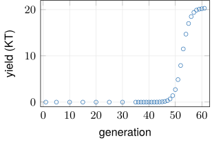
(b) Estimate the four parameters by the method of the Lesson 9 sheet, section 4. The figure marks each estimate on the readings from generation 40 on: the two levels and , the halfway point at the mean , and the spread as the input distance from to the five-sixths level.

- The vertical shift is the level on the left, near 0 where the readings start: .
- The amplitude is the whole rise from the level on the left to the level on the right. The last four readings, from 19.90 to 20.30, sit near the level 20: .
The mean is the input at the halfway output . The readings are 7.92 at generation 52 and 11.50 at generation 53. The output 10 lies of the way between them:
The estimate of the spread is the input distance from to the five-sixths level , which stands in for the
pnorm(1)point (Lesson 9 sheet, section 2). The readings are 14.70 at generation 54 and 17.00 at generation 55. The output 16.7 lies of the way between them, at about generation :
(c) Fit the sigmoid model as on the Lesson 9 sheet, section 5, with the hand estimates as the start values:
generation = c(1, 5, 10, 15, 20, 25, 30, 35,
36, 37, 38, 39, 40, 41, 42, 43,
44, 45, 46, 47, 48, 49, 50, 51)
yield_KT = c(6.66e-18, 3.12e-16, 1.93e-14, 1.19e-12,
7.32e-11, 4.54e-9, 2.83e-7, 1.78e-5, 4.07e-5,
9.31e-5, 2.13e-4, 4.88e-4, 1.11e-3, 2.55e-3,
5.80e-3, 0.0132, 0.0298, 0.0668, 0.148, 0.323,
0.685, 1.40, 2.71, 4.87)
generation2 = c(generation, 52, 53, 54, 55, 56,
57, 58, 59, 60, 61)
yield_KT2 = c(yield_KT, 7.92, 11.5, 14.7, 17.0,
18.5, 19.4, 19.9, 20.1, 20.2, 20.3)
bomb2 = fitModel(yield_KT2 ~ A*pnorm(generation2, m, s) + v,
start = list(A = 20, m = 52.6, s = 2.3, v = 0))
coef(bomb2)
The last line prints , , , and . The best-fit model is
(d) The fitModel() call in part (c) stores bomb2. Draw bomb2 over all 34 readings:
=2.2em plotPoints(yield_KT2 ~ generation2)
plotFun(bomb2(generation2) ~
generation2, add = TRUE, col = "red")
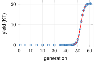
The red curve is the model, drawn with col = "red". It lies within 0.17 kilotons of every reading, at both levels and along the rise between them.
Example 5
Use the sigmoid model of Example 4 to predict the yield at generations 47 and 53. Classify each prediction as an interpolation or an extrapolation, and compare each with the reading at that generation.
ShowHide solution
Rebuild the sigmoid model of Example 4 and evaluate it at generations 47 and 53:
generation = c(1, 5, 10, 15, 20, 25, 30, 35,
36, 37, 38, 39, 40, 41, 42, 43,
44, 45, 46, 47, 48, 49, 50, 51)
yield_KT = c(6.66e-18, 3.12e-16, 1.93e-14, 1.19e-12,
7.32e-11, 4.54e-9, 2.83e-7, 1.78e-5, 4.07e-5,
9.31e-5, 2.13e-4, 4.88e-4, 1.11e-3, 2.55e-3,
5.80e-3, 0.0132, 0.0298, 0.0668, 0.148, 0.323,
0.685, 1.40, 2.71, 4.87)
generation2 = c(generation, 52, 53, 54, 55, 56,
57, 58, 59, 60, 61)
yield_KT2 = c(yield_KT, 7.92, 11.5, 14.7, 17.0,
18.5, 19.4, 19.9, 20.1, 20.2, 20.3)
bomb2 = fitModel(yield_KT2 ~ A*pnorm(generation2, m, s) + v,
start = list(A = 20, m = 52.6, s = 2.3, v = 0))
bomb2(47)
bomb2(53)
R returns predictions of kilotons at generation 47 and kilotons at generation 53. Both predictions are interpolations, because 47 and 53 lie inside generations 1 to 61, the inputs of all 34 readings. At generation 53 the reading is 11.50, and the model is within 1 percent of it. At generation 47 the reading is 0.323, and the model is 37 percent low.
Example 6
Determine the first generation at which the sigmoid model of Example 4 gives a yield of at least 10 kilotons.
ShowHide solution
Evaluate the model at generations 52 and 53, where the readings cross 10 kilotons:
generation = c(1, 5, 10, 15, 20, 25, 30, 35,
36, 37, 38, 39, 40, 41, 42, 43,
44, 45, 46, 47, 48, 49, 50, 51)
yield_KT = c(6.66e-18, 3.12e-16, 1.93e-14, 1.19e-12,
7.32e-11, 4.54e-9, 2.83e-7, 1.78e-5, 4.07e-5,
9.31e-5, 2.13e-4, 4.88e-4, 1.11e-3, 2.55e-3,
5.80e-3, 0.0132, 0.0298, 0.0668, 0.148, 0.323,
0.685, 1.40, 2.71, 4.87)
generation2 = c(generation, 52, 53, 54, 55, 56,
57, 58, 59, 60, 61)
yield_KT2 = c(yield_KT, 7.92, 11.5, 14.7, 17.0,
18.5, 19.4, 19.9, 20.1, 20.2, 20.3)
bomb2 = fitModel(yield_KT2 ~ A*pnorm(generation2, m, s) + v,
start = list(A = 20, m = 52.6, s = 2.3, v = 0))
bomb2(52)
bomb2(53)
R returns kilotons at generation 52, below 10, and kilotons at generation 53, above 10. The model is increasing, because pnorm increases with generation and is positive. So the first generation with a yield of at least 10 kilotons is generation 53.