Lesson 22: The Method of Least Squares I

Objectives

Use least squares to obtain the best-fit linear model for a dataset.
Given a dataset and a linear model, compute the residual vector.
Given a residual vector, compute its length and the associated RMSE.

1. Best-Fit Linear Model

Objective. Use least squares to obtain the best-fit linear model for a dataset.

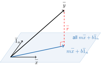
A dataset with $n$ points $(x_1, y_1), \dots, (x_n, y_n)$ is stored as an input vector $\overline{\vphantom{b}x}$ and a target vector $\overline{\vphantom{b}y}$ . The intercept vector $\overline{\vphantom{b}1}_n$ of Lesson 19 is the vector of $n$ ones. When every point lies on one line $y = mx + b$ , the vector equation

\overline{\vphantom{b}y} = m\overline{\vphantom{b}x} + b\overline{\vphantom{b}1}_n

has a solution. When no line $y = mx + b$ passes through every point, no linear combination of $\overline{\vphantom{b}x}$ and $\overline{\vphantom{b}1}_n$ equals $\overline{\vphantom{b}y}$ .

When the entries of $\overline{\vphantom{b}x}$ are not all equal, the linear combinations $m\overline{\vphantom{b}x} + b\overline{\vphantom{b}1}_n$ fill a plane, shaded in the figure. The residual vector $\overline{\vphantom{b}r}$ runs from the point of that plane closest to $\overline{\vphantom{b}y}$ to the tip of the target vector $\overline{\vphantom{b}y}$ and meets the plane at a right angle.

Definition 1 (Method of least squares).

The method of least squares is the method that selects the linear combination $m\overline{\vphantom{b}x} + b\overline{\vphantom{b}1}_n$ closest to the target vector $\overline{\vphantom{b}y}$ , in the sense that the corresponding residual vector $\overline{\vphantom{b}r} = \overline{\vphantom{b}y} - (m\overline{\vphantom{b}x} + b\overline{\vphantom{b}1}_n)$ has the shortest length possible. When the entries of $\overline{\vphantom{b}x}$ are not all equal, it selects one pair of scalars $m$ and $b$ , the slope and the vertical intercept of the best-fit linear model $y = mx + b$ .

The data $(2, 1)$ , $(2, 3)$ , and $(2, 5)$ fail the condition of the definition that the entries of $\overline{\vphantom{b}x}$ are not all equal, and they have no single best-fit linear model. Every entry of $\overline{\vphantom{b}x} = \left(\begin{smallmatrix} 2\\2\\2 \end{smallmatrix}\right)$ equals 2. As a result, every combination $m\overline{\vphantom{b}x} + b\overline{\vphantom{b}1}_3 = (2m + b)\overline{\vphantom{b}1}_3$ is a multiple of $\overline{\vphantom{b}1}_3$ . The multiple of $\overline{\vphantom{b}1}_3$ closest to $\overline{\vphantom{b}y} = \left(\begin{smallmatrix} 1\\3\\5 \end{smallmatrix}\right)$ is the projection of $\overline{\vphantom{b}y}$ onto $\overline{\vphantom{b}1}_3$ (Lesson 21):

\frac{\overline{\vphantom{b}y}\cdot\overline{\vphantom{b}1}_3}{\overline{\vphantom{b}1}_3\cdot\overline{\vphantom{b}1}_3}\,\overline{\vphantom{b}1}_3 = \frac{1 + 3 + 5}{3}\,\overline{\vphantom{b}1}_3 = 3\,\overline{\vphantom{b}1}_3 = \left(\begin{smallmatrix} 3\\3\\3 \end{smallmatrix}\right).

Every pair with $2m + b = 3$ gives this closest vector. The method therefore has no single pair to select.

The linear combination $m\overline{\vphantom{b}x} + b\overline{\vphantom{b}1}_n$ that the method of least squares selects is the model vector, the vector of the model’s predictions.

As with the projection onto one vector (Lesson 21), the least squares residual vector is orthogonal to $\overline{\vphantom{b}x}$ , to $\overline{\vphantom{b}1}_n$ , and to the model vector. In the figure, $\overline{\vphantom{b}r}$ meets the shaded plane at a right angle.

Least squares in R. Each command below carries out the method of least squares, and the right column gives what it returns. In project(), the 1 stands for the intercept vector.

project(y ~ x + 1)
returns  $b$ , then  $m$ 
coef(fitModel(y ~ m*x + b))
returns  $m$ , then  $b$ 
project(output ~ input + 1, data = Name)
returns  $b$ , then  $m$ , for an MMAC dataset

Model with no intercept. The command project(y ~ x) returns a single number, the slope of the best-fit linear model through the origin, $y = mx$ . That model fixes $b$ at 0, where the method of least squares chooses $b$ freely. When the entries of $\overline{\vphantom{b}x}$ are not all equal, the residual vector of the model through the origin is longer than the least squares residual vector unless the best-fit intercept $b$ is 0.

Example 1

The table gives the number of Twitter users, in millions, by quarter. Year counts years since 2000. The value 11 is January to March 2011. Use the method of least squares in R to find the best-fit linear model $\text{Users} = m\,\text{Year} + b$ .

Year	11	11.25	11.5	11.75	12.75
Users	68	85	101	117	185

ShowHide solution

By the definition of the method of least squares, the best-fit $m$ and $b$ make the residual vector $\overline{\vphantom{b}\text{Users}} - (m\,\overline{\vphantom{b}\text{Year}} + b\overline{\vphantom{b}1}_5)$ as short as possible. Store the data as vectors and compute $m$ and $b$ with project():

Year = c(11, 11.25, 11.5, 11.75, 12.75)
Users = c(68, 85, 101, 117, 185)
project(Users ~ Year + 1)
(Intercept)        Year
-666.63699    66.76712

In the command, Year stands for $\overline{\vphantom{b}\text{Year}}$ and 1 for the intercept vector $\overline{\vphantom{b}1}_5$ . R prints $b$ under (Intercept) and $m$ under the input’s name. The best-fit linear model is

\text{Users} = 66.767\,\text{Year} - 666.637.

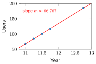
Each column of the table is one blue point $(\text{Year}, \text{Users})$ , and the red line is the best-fit linear model, with slope $m \approx 66.767$ : the model’s prediction rises about 66.767 million users per year.

Package datasets. With data =, R reads the columns of an MMAC dataset. Without data =, R looks in the session for vectors named like the formula’s variables. When those vectors exist, R fits them without an error.

With the vectors of Example 1 in the session, the two commands below fit different data. The first fits all 17 quarters of the MMAC dataset TwitterUsers, and the second fits the five values typed in Example 1:

> project(Users ~ Year + 1, data = TwitterUsers)
(Intercept)        Year
-584.21765    60.12941
> project(Users ~ Year + 1)
(Intercept)        Year
-666.63699    66.76712

If no vectors named Users and Year exist, the second command stops with an error:

> project(Users ~ Year + 1)
Error in eval(predvars, data, env) : object 'Users' not found

Example 2

The MMAC dataset HealthExpenditure records United States health expenditure as a percent of gross domestic product, PercentGDP, for each Year from 1995 to 2012. Use the method of least squares to find the best-fit linear model of PercentGDP as a function of Year.

ShowHide solution

Run the method of least squares with project(), reading the columns with data =, and print the result:

cf = project(PercentGDP ~ Year + 1, data = HealthExpenditure)
cf
(Intercept)         Year
-585.2139570    0.2997804

Reading $b$ and $m$ as in Example 1 and rounding to three decimals, the best-fit linear model is

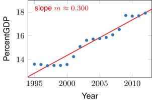
\text{PercentGDP} = 0.300\,\text{Year} - 585.214.

Each row of the dataset is one blue point $(\text{Year}, \text{PercentGDP})$ , and the red line is the model, with slope $m \approx 0.300$ : the prediction rises about 0.300 percentage points per year.

Next: 2. Residual Vector Lesson map

2. Residual Vector

Objective. Given a dataset and a linear model, compute the residual vector.

For the linear model $y = mx + b$ , the residual vector (Lesson 21) is the target vector minus the linear combination $m\overline{\vphantom{b}x} + b\overline{\vphantom{b}1}_n$ :

\overline{\vphantom{b}r} = \overline{\vphantom{b}y} - (m\overline{\vphantom{b}x} + b\overline{\vphantom{b}1}_n).

Component $i$ is

r_i = y_i - (mx_i + b),

the data value minus the model’s prediction, in the units of the output.

Sign of a residual. The sign of $r_i$ places data point $i$ relative to the line. In each graph below, the red line is the model and the segment is $r_i$ .

Positive residual

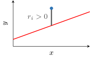
The data value $y_i$ exceeds the prediction $mx_i + b$ , and the point lies above the line. In the Twitter data of Example 1, a quarter with a positive residual had more users than the model predicts.

Negative residual

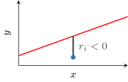
The data value $y_i$ is less than the prediction $mx_i + b$ , and the point lies below the line. A quarter with a negative residual had fewer users than the model predicts.

Zero residual

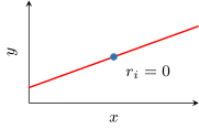
The data value $y_i$ equals the prediction $mx_i + b$ , and the point lies on the line. A quarter with a zero residual had exactly the number of users the model predicts.

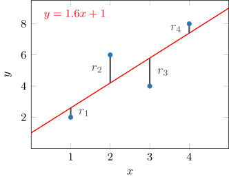
Residuals on a plot. The residual $r_i$ is the signed length of the vertical segment between data point $i$ and the line. In the plot below, the best-fit linear model for the four data points is $y = 1.6x + 1$ . Each residual is the data value minus the line’s value at that input, as in $r_1 = 2 - (1.6(1) + 1) = -0.6$ , and the residual vector lists the four residuals in order.

\overline{\vphantom{b}r} = \begin{pmatrix*}[r] r_1 \\ r_2 \\ r_3 \\ r_4 \end{pmatrix*} = \begin{pmatrix*}[r] -0.6 \\ 1.8 \\ -1.8 \\ 0.6 \end{pmatrix*}.

Rounding. Compute predictions and residuals from the stored fit. To store the fit, save the $b$ and $m$ that project() returns at full precision and build the model from them, as the commands below do for the Twitter data of Example 1. The entry cf[1] is the first number project() returns, $b$ , and cf[2] is the second, $m$ .

Year = c(11, 11.25, 11.5, 11.75, 12.75)
Users = c(68, 85, 101, 117, 185)
cf = project(Users ~ Year + 1)
b = cf[1]
m = cf[2]
f = makeFun(m*Year + b ~ Year)

With the fit stored, the model vector is f(Year) and the residual vector is Users - f(Year).

Rounded coefficients can move a prediction far more than the rounding itself. A change in the slope $m$ changes each prediction by that change times the input, and a calendar year multiplies a slope change by about 2000. For the HealthExpenditure fit of Example 2, R prints $b = -585.2139570$ and $m = 0.2997804$ . Rounding the slope to $m = 0.300$ changes it by only 0.0002196, yet it raises the 2005 prediction by about 0.440 percentage points. With both coefficients rounded to three decimals, the residual vector has length 2.519, against 1.691 for the stored fit.

Example 3

The best-fit linear model for the data below, with exact coefficients, is

y = \frac{40}{13}x + \frac{29}{13}.

Compute the residual vector by hand and interpret its third component.

$x$	$-1$	2	3
$y$	$-1$	9	11

ShowHide solution

By the definition of the residual vector, $\overline{\vphantom{b}r}$ is the target vector minus the model’s predictions, here with $n = 3$ :

\overline{\vphantom{b}r} = \overline{\vphantom{b}y} - (m\overline{\vphantom{b}x} + b\overline{\vphantom{b}1}_3).

Substitute $m = 40/13$ , $b = 29/13$ , and the inputs into $m\overline{\vphantom{b}x} + b\overline{\vphantom{b}1}_3$ . The model’s predictions, kept as fractions, are

\frac{40}{13}\begin{pmatrix*}[r] -1 \\ 2 \\ 3 \end{pmatrix*} + \frac{29}{13}\begin{pmatrix*}[r] 1 \\ 1 \\ 1 \end{pmatrix*} = \frac{1}{13}\begin{pmatrix*}[r] -40 + 29 \\ 80 + 29 \\ 120 + 29 \end{pmatrix*} = \frac{1}{13}\begin{pmatrix*}[r] -11 \\ 109 \\ 149 \end{pmatrix*},

so the residual vector, with $\overline{\vphantom{b}y}$ written over 13, is

\overline{\vphantom{b}r} = \frac{1}{13}\begin{pmatrix*}[r] -13 \\ 117 \\ 143 \end{pmatrix*} - \frac{1}{13}\begin{pmatrix*}[r] -11 \\ 109 \\ 149 \end{pmatrix*} = \frac{1}{13}\begin{pmatrix*}[r] -2 \\ 8 \\ -6 \end{pmatrix*} \approx \begin{pmatrix*}[r] -0.154 \\ 0.615 \\ -0.462 \end{pmatrix*}.

The third component, $-6/13$ , is negative: the point $(3, 11)$ lies $6/13 \approx 0.462$ below the line.

Example 4

For the best-fit linear model of Example 1, with Year $= 11, 11.25, 11.5, 11.75, 12.75$ and Users $= 68, 85, 101, 117, 185$ , compute the residual vector in R and interpret its fourth component.

ShowHide solution

Store the fit from project() at full precision and subtract its predictions from Users:

Year = c(11, 11.25, 11.5, 11.75, 12.75)
Users = c(68, 85, 101, 117, 185)
cf = project(Users ~ Year + 1)
b = cf[1]
m = cf[2]
f = makeFun(m*Year + b ~ Year)
r = Users - f(Year)
r
[1]  0.1986301  0.5068493 -0.1849315 -0.8767123  0.3561644

The line r = Users - f(Year) computes $\overline{\vphantom{b}r} = \overline{\vphantom{b}\text{Users}} - (m\,\overline{\vphantom{b}\text{Year}} + b\overline{\vphantom{b}1}_5)$ , and R prints its five components in the order of the table, one per quarter. The fourth component, about $-0.877$ , is the residual for Year $= 11.75$ . It means Twitter had about 0.877 million fewer users in October to December 2011 than the model predicts.

Next: 3. Length of the Residual Vector and RMSE Lesson map

3. Length of the Residual Vector and RMSE

Objective. Given a residual vector, compute its length and the associated RMSE.

The length of a residual vector is

\|\overline{\vphantom{b}r}\| = \sqrt{\overline{\vphantom{b}r}\cdot\overline{\vphantom{b}r}},

as for every vector (Lesson 20). In R, sqrt(dot(r, r)) computes the length.

Definition 2 (Root mean squared error (RMSE)).

For a model fit to $n$ data points, the root mean squared error (RMSE) is the square root of the mean of the squared components of its residual vector $\overline{\vphantom{b}r}$ :

\text{RMSE} = \frac{\|\overline{\vphantom{b}r}\|}{\sqrt{n}} = \sqrt{\frac{\|\overline{\vphantom{b}r}\|^2}{n}}.

For a residual vector with the two components 1 and $-1$ , the mean of the components is 0, yet the RMSE is $\sqrt{(1^2 + (-1)^2)/2} = 1$ . The RMSE squares each component before it takes the mean. As a result, positive and negative residuals do not cancel.

For a fixed model, the length $\|\overline{\vphantom{b}r}\|$ never shrinks as data points are added, because each added data point puts one more squared residual under the square root. Dividing $\|\overline{\vphantom{b}r}\|^2$ by $n$ removes that growth: the quotient is the mean of the squared residuals. Its square root, the RMSE, measures the typical size of one residual, in the units of the output.

Because $\sqrt{n} \ge 1$ , the RMSE is never larger than the length $\|\overline{\vphantom{b}r}\|$ . For the same data, a smaller RMSE means the model’s predictions lie closer to the data values, on average.

Proposition 3 (Least squares RMSE).

When the entries of $\overline{\vphantom{b}x}$ are not all equal, the best-fit linear model has the smallest RMSE of all linear models $y = mx + b$ for the same data.

The least squares RMSE proposition follows from $\text{RMSE} = \|\overline{\vphantom{b}r}\|/\sqrt{n}$ . For the same data, $n$ is fixed, and the method of least squares gives the shortest residual vector.

Example 5

Compute the length of the residual vector from Example 3 and the associated RMSE:

\overline{\vphantom{b}r} = \frac{1}{13}\begin{pmatrix*}[r] -2 \\ 8 \\ -6 \end{pmatrix*}.

ShowHide solution

Use the formula for the length of a vector and the definition of RMSE:

\|\overline{\vphantom{b}r}\| = \sqrt{\overline{\vphantom{b}r}\cdot\overline{\vphantom{b}r}}, \qquad \text{RMSE} = \frac{\|\overline{\vphantom{b}r}\|}{\sqrt{n}}.

With the components of $\overline{\vphantom{b}r}$ ,

\|\overline{\vphantom{b}r}\| = \sqrt{\left(\frac{-2}{13}\right)^2 + \left(\frac{8}{13}\right)^2 + \left(\frac{-6}{13}\right)^2} = \sqrt{\frac{4 + 64 + 36}{169}} = \sqrt{\frac{104}{169}} \approx 0.784,

and with $n = 3$ data points,

\text{RMSE} = \frac{\sqrt{104/169}}{\sqrt{3}} = \sqrt{\frac{104}{507}} \approx 0.453.

Example 6

For the best-fit linear model of Example 1, with Year $= 11, 11.25, 11.5, 11.75, 12.75$ and Users $= 68, 85, 101, 117, 185$ , compute the length of the residual vector and the RMSE in R.

ShowHide solution

R computes the residual vector, its length, and the RMSE with $n = 5$ data points:

Year = c(11, 11.25, 11.5, 11.75, 12.75)
Users = c(68, 85, 101, 117, 185)
cf = project(Users ~ Year + 1)
b = cf[1]
m = cf[2]
f = makeFun(m*Year + b ~ Year)
r = Users - f(Year)
r.length = sqrt(dot(r, r))
r.length
[1] 1.107261
rmse = r.length/sqrt(5)
rmse
[1] 0.4951823

The line for r.length computes $\|\overline{\vphantom{b}r}\| = \sqrt{\overline{\vphantom{b}r}\cdot\overline{\vphantom{b}r}}$ , and the line for rmse divides it by $\sqrt{n}$ with $n = 5$ . The length is $\|\overline{\vphantom{b}r}\| \approx 1.107$ . The RMSE is about 0.495 million users, small beside outputs that run from 68 to 185 million.

Example 7

For the Twitter data with Year $= 11, 11.25, 11.5, 11.75, 12.75$ and Users $= 68, 85, 101, 117, 185$ , consider the line of MMAC Section 3.5, Example 3, and the line through the first two data points (Lesson 20, Example 7):

\text{Users} = 66\,\text{Year} - 657.7, \qquad\qquad \text{Users} = 68\,\text{Year} - 680.

Use R to compare the lengths of their residual vectors with the length of the least squares residual vector, about 1.107.

ShowHide solution

Compute each line’s residual vector, Users minus the line’s predictions, and its length:

Year = c(11, 11.25, 11.5, 11.75, 12.75)
Users = c(68, 85, 101, 117, 185)
r2 = Users - (66*Year - 657.7)
r2
[1] -0.3  0.2 -0.3 -0.8  1.2
sqrt(dot(r2, r2))
[1] 1.516575
r3 = Users - (68*Year - 680)
r3
[1]  0  0 -1 -2 -2
sqrt(dot(r3, r3))
[1] 3

The residual vector of the MMAC line has length about 1.517, and the residual vector of the two-point line has length 3. Both are longer than the least squares residual vector, of length about 1.107, as the definition of the method of least squares guarantees.

Lesson map