Lesson 18: Matrix Equations

Objectives

Rewrite a vector equation as an equivalent matrix equation (and vice-versa).
In R, use matrix() to define a matrix.
Rewrite a system of equations as an equivalent matrix equation (and vice-versa).
In R, use solve() to find the solution of a matrix equation.

1. Vector Equations as Matrix Equations

Objective. Rewrite a vector equation as an equivalent matrix equation (and vice-versa).

The vector equation and the matrix equation are equivalent,

x\begin{pmatrix*}[r] -3 \\ 2 \end{pmatrix*} + y\begin{pmatrix*}[r] 1 \\ 4 \end{pmatrix*} = \begin{pmatrix*}[r] 15 \\ 18 \end{pmatrix*}, \qquad \begin{pmatrix*}[r] 15 \\ 18 \end{pmatrix*} = \begin{pmatrix*}[r] -3 & 1 \\ 2 & 4 \end{pmatrix*}\begin{pmatrix*}[r] x \\ y \end{pmatrix*},

because the matrix-vector product on the right is $x\left(\begin{smallmatrix} -3\\2 \end{smallmatrix}\right) + y\left(\begin{smallmatrix} 1\\4 \end{smallmatrix}\right)$ . Matrices, their sizes, and the matrix-vector product are on the Lesson 17 sheet, sections 5 and 6.

Definition 1 (Matrix equation).

A matrix equation is an equation $\overline{\vphantom{b}v} = U\overline{\vphantom{b}x}$ in which a matrix $U$ times the vector of unknowns $\overline{\vphantom{b}x}$ equals a known vector $\overline{\vphantom{b}v}$ . The columns of $U$ are vectors $\overline{\vphantom{b}u}_1, \overline{\vphantom{b}u}_2, \dots, \overline{\vphantom{b}u}_n$ , all of the same dimension $m$ as $\overline{\vphantom{b}v}$ , so that

U = \begin{pmatrix*}[r] \overline{\vphantom{b}u}_1 & \overline{\vphantom{b}u}_2 & \cdots & \overline{\vphantom{b}u}_n \end{pmatrix*}, \qquad \overline{\vphantom{b}x} = \begin{pmatrix*}[r] x_1 \\ x_2 \\ \vdots \\ x_n \end{pmatrix*}, \qquad U\overline{\vphantom{b}x} = x_1\overline{\vphantom{b}u}_1 + x_2\overline{\vphantom{b}u}_2 + \cdots + x_n\overline{\vphantom{b}u}_n.

The known vector $\overline{\vphantom{b}v}$ is the target vector.

The two sides may be written in either order: the equations $\overline{\vphantom{b}v} = U\overline{\vphantom{b}x}$ and $U\overline{\vphantom{b}x} = \overline{\vphantom{b}v}$ are the same equation.

The equation

\begin{pmatrix*}[r] 1 & 2 \\ 3 & 4 \end{pmatrix*}\begin{pmatrix*}[r] x \\ y \end{pmatrix*} = \begin{pmatrix*}[r] 5 \\ 6 \\ 7 \end{pmatrix*}

is not a matrix equation, because the columns of its matrix have two components and its target vector has three. The definition requires every column to have the same dimension $m$ as $\overline{\vphantom{b}v}$ .

Vector equation to matrix equation.

Write the vector that each unknown multiplies as one column of the matrix, in the order of the unknowns.
List the unknowns, in the same order, as the vector of unknowns.
Write the remaining vector as the target vector.

Matrix equation to vector equation.

Multiply column $i$ of the matrix by component $i$ of the vector of unknowns.
Add the products. The sum is the linear combination on one side.
Write the target vector on the other side.

The size of the matrix follows from the equation: the matrix has one row for each component of $\overline{\vphantom{b}v}$ and one column for each unknown.

Example 1

Rewrite the vector equation of MMAC Example 5 as a matrix equation:

\begin{pmatrix*}[r] 4 \\ -1 \\ 3 \end{pmatrix*} = x_1\begin{pmatrix*}[r] 1 \\ -2 \\ 1 \end{pmatrix*} + x_2\begin{pmatrix*}[r] 4 \\ 8 \\ -7 \end{pmatrix*} + x_3\begin{pmatrix*}[r] 5 \\ 1 \\ 0 \end{pmatrix*}.

ShowHide solution

By the definition of a matrix equation, the columns of the matrix are the vectors that the unknowns multiply, in the order of $x_1$ , $x_2$ , and $x_3$ , and the vector of unknowns lists $x_1$ , $x_2$ , and $x_3$ in that order:

\begin{pmatrix*}[r] 4 \\ -1 \\ 3 \end{pmatrix*} = \begin{pmatrix*}[r] 1 & 4 & 5 \\ -2 & 8 & 1 \\ 1 & -7 & 0 \end{pmatrix*}\begin{pmatrix*}[r] x_1 \\ x_2 \\ x_3 \end{pmatrix*}.

Example 2

Rewrite the matrix equation as a vector equation, and give the size of its matrix:

\begin{pmatrix*}[r] 2 & 1 \\ 0 & -3 \\ 4 & 5 \end{pmatrix*}\begin{pmatrix*}[r] a \\ b \end{pmatrix*} = \begin{pmatrix*}[r] 5 \\ 3 \\ 7 \end{pmatrix*}.

ShowHide solution

Multiply each column of the matrix by its own unknown:

a\begin{pmatrix*}[r] 2 \\ 0 \\ 4 \end{pmatrix*} + b\begin{pmatrix*}[r] 1 \\ -3 \\ 5 \end{pmatrix*} = \begin{pmatrix*}[r] 5 \\ 3 \\ 7 \end{pmatrix*}.

The matrix is $3 \times 2$ : three rows, because each vector has three components, and two columns, one for each unknown.

Example 3

Rewrite the matrix equation as a vector equation:

\begin{pmatrix*}[r] 4 & -1 & 0 \\ 2 & 3 & 5 \\ -6 & 1 & 2 \end{pmatrix*}\begin{pmatrix*}[r] p \\ q \\ r \end{pmatrix*} = \begin{pmatrix*}[r] 7 \\ 0 \\ -3 \end{pmatrix*}.

ShowHide solution

Multiplying each column of the matrix by its own unknown gives the vector equation

p\begin{pmatrix*}[r] 4 \\ 2 \\ -6 \end{pmatrix*} + q\begin{pmatrix*}[r] -1 \\ 3 \\ 1 \end{pmatrix*} + r\begin{pmatrix*}[r] 0 \\ 5 \\ 2 \end{pmatrix*} = \begin{pmatrix*}[r] 7 \\ 0 \\ -3 \end{pmatrix*}.

Example 4

A strike takes 28 missiles and 40 bombs. Each B-1B sortie carries 8 missiles and 16 bombs, and each B-52H sortie carries 12 missiles and 8 bombs. With $x$ B-1B sorties and $y$ B-52H sorties, the tasking is the vector equation

x\begin{pmatrix*}[r] 8 \\ 16 \end{pmatrix*} + y\begin{pmatrix*}[r] 12 \\ 8 \end{pmatrix*} = \begin{pmatrix*}[r] 28 \\ 40 \end{pmatrix*}.

Rewrite it as a matrix equation, and state what each column and each row of the matrix counts.

ShowHide solution

The vector that each unknown multiplies becomes one column of the matrix, in the order of $x$ and $y$ :

\begin{pmatrix*}[r] 8 & 12 \\ 16 & 8 \end{pmatrix*}\begin{pmatrix*}[r] x \\ y \end{pmatrix*} = \begin{pmatrix*}[r] 28 \\ 40 \end{pmatrix*}.

Column 1 is the load of one B-1B sortie, and column 2 is the load of one B-52H sortie. Row 1 counts missiles, and row 2 counts bombs, the same order as the target vector.

Next: 2. Defining a Matrix in R Lesson map

2. Defining a Matrix in R

Objective. In R, use matrix() to define a matrix.

The command matrix(c(...), nrow = m, ncol = n) defines a matrix with $m$ rows and $n$ columns from a list of exactly $m \cdot n$ entries. R fills the columns in order and each column from top to bottom.

`U = matrix(c(-3, 2, 1, 4), nrow = 2, ncol = 2)`
`U`	the matrix’s name
`c(-3, 2, 1, 4)`	the entries: column 1, then column 2
`nrow = 2`	the number of rows
`ncol = 2`	the number of columns

To print the matrix, type the name U on its own line. R labels the rows [1,] and [2,] and the columns [,1] and [,2]:

  [,1]  [,2]
[1,]  -3  1
[2,]  2  4

Print every matrix before using it, and compare it with the matrix on paper.

Columns stored as vectors. When the columns are already stored as vectors, c() joins them in order. The last line defines the matrix $\left(\begin{smallmatrix} -3 & 1\\2 & 4 \end{smallmatrix}\right)$ :

u1 = c(-3, 2)
u2 = c(1, 4)
U = matrix(c(u1, u2), nrow = 2, ncol = 2)

Entries typed across the rows. The call matrix(c(-3, 1, 2, 4), nrow = 2, ncol = 2) still fills down the columns and defines $\left(\begin{smallmatrix} -3 & 2\\1 & 4 \end{smallmatrix}\right)$ , whose columns are the rows of the intended matrix $\left(\begin{smallmatrix} -3 & 1\\2 & 4 \end{smallmatrix}\right)$ .

Entries inside one c(). Every entry goes inside the one c(), because matrix() reads its first input as the entries, its second as the number of rows, and its third as the number of columns. When the call matrix(-3, 2, 1, 4) leaves out the c(), R takes $-3$ as the only entry, 2 as the number of rows, and 1 as the number of columns. R reads the fourth input, 4, as a setting for the fill order, which changes nothing for a single entry. The call returns a $2 \times 1$ matrix of $-3$ s with no error message, and the mistake appears only in the printout:

  [,1]
[1,]  -3
[2,]  -3

Example 5

Use matrix() to define the matrix $B$ of Example 2 from its columns, then print it:

B = \begin{pmatrix*}[r] 2 & 1 \\ 0 & -3 \\ 4 & 5 \end{pmatrix*}.

ShowHide solution

Store the two columns of $B$ as vectors, join them in matrix(), and print $B$ :

b1 = c(2, 0, 4)
b2 = c(1, -3, 5)
B = matrix(c(b1, b2), nrow = 3, ncol = 2)
B

The last line prints

  [,1]  [,2]
[1,]  2  1
[2,]  0  -3
[3,]  4  5

The call matrix(c(b1, b2), nrow = 2, ncol = 3) reverses the two sizes and defines the $2 \times 3$ matrix $\left(\begin{smallmatrix} 2 & 4 & -3\\0 & 1 & 5 \end{smallmatrix}\right)$ , a different matrix from $B$ .

Example 6

Use matrix() to define the matrix of Example 1 by listing its entries, then print it:

\begin{pmatrix*}[r] 1 & 4 & 5 \\ -2 & 8 & 1 \\ 1 & -7 & 0 \end{pmatrix*}.

ShowHide solution

The entries go in column by column: $1, -2, 1$ , then $4, 8, -7$ , then $5, 1, 0$ .

U = matrix(c(1, -2, 1, 4, 8, -7, 5, 1, 0), nrow = 3, ncol = 3)
U

The last line prints

  [,1]  [,2]  [,3]
[1,]  1  4  5
[2,]  -2  8  1
[3,]  1  -7  0

Next: 3. Systems as Matrix Equations Lesson map

3. Systems as Matrix Equations

Objective. Rewrite a system of equations as an equivalent matrix equation (and vice-versa).

A system of linear equations has an equivalent vector equation and an equivalent matrix equation. The table shows one system in all three forms. The matrix has one row per equation and one column per unknown.

System	Vector equation	Matrix equation
$\begin{aligned} -3x + y &= 15 \\ 2x + 4y &= 18 \end{aligned}$	$x\begin{pmatrix}[r] -3 \\ 2 \end{pmatrix} + y\begin{pmatrix}[r] 1 \\ 4 \end{pmatrix} = \begin{pmatrix}[r] 15 \\ 18 \end{pmatrix}$	$\begin{pmatrix}[r] 15 \\ 18 \end{pmatrix} = \begin{pmatrix}[r] -3 & 1 \\ 2 & 4 \end{pmatrix}\begin{pmatrix}[r] x \\ y \end{pmatrix}$

System to matrix equation.

Write every equation with the unknowns on the left, in the same order, and the constant on the right. An equation with no constant has 0 on the right.
Write a 0 coefficient wherever an unknown is missing.
Copy the coefficients of equation $i$ into row $i$ of the matrix.
List the unknowns, in order, as the vector of unknowns, and the constants as the target vector.

Matrix equation to system.

Multiply each entry of row $i$ by its unknown, and add the products. The sum is the left side of equation $i$ .
Leave out of equation $i$ every unknown whose entry in row $i$ is 0.
Write component $i$ of the target vector as the right side of equation $i$ .

Example 7

Rewrite the system as a matrix equation:

\begin{aligned} 2x + z &= 5 \\ 4y - z &= 1 \\ 3x + y &= 4. \end{aligned}

ShowHide solution

Equation 1 has no $y$ , equation 2 has no $x$ , and equation 3 has no $z$ . Each missing unknown takes the coefficient 0 in its row of the matrix:

\begin{pmatrix*}[r] 2 & 0 & 1 \\ 0 & 4 & -1 \\ 3 & 1 & 0 \end{pmatrix*}\begin{pmatrix*}[r] x \\ y \\ z \end{pmatrix*} = \begin{pmatrix*}[r] 5 \\ 1 \\ 4 \end{pmatrix*}.

Example 8

Rewrite the system as a matrix equation:

\begin{aligned} 4x &= 7 - 2y + z \\ y - 3z &= x + 1 \\ 5z &= 2x. \end{aligned}

ShowHide solution

Move every unknown to the left side, in the order $x$ , $y$ , $z$ , and write the 0 for the missing $y$ in equation 3:

\begin{aligned} 4x + 2y - z &= 7 \\ -x + y - 3z &= 1 \\ -2x + 0y + 5z &= 0. \end{aligned}

Copy the coefficients of each equation into its row of the matrix:

\begin{pmatrix*}[r] 4 & 2 & -1 \\ -1 & 1 & -3 \\ -2 & 0 & 5 \end{pmatrix*}\begin{pmatrix*}[r] x \\ y \\ z \end{pmatrix*} = \begin{pmatrix*}[r] 7 \\ 1 \\ 0 \end{pmatrix*}.

Example 9

Rewrite the matrix equation as a system of equations:

\begin{pmatrix*}[r] 1 & 0 & -2 \\ 3 & 1 & 0 \\ 0 & -4 & 5 \end{pmatrix*}\begin{pmatrix*}[r] x \\ y \\ z \end{pmatrix*} = \begin{pmatrix*}[r] 6 \\ -1 \\ 2 \end{pmatrix*}.

ShowHide solution

Each row gives one equation:

\begin{aligned} x - 2z &= 6 \\ 3x + y &= -1 \\ -4y + 5z &= 2. \end{aligned}

Example 10

Rewrite the matrix equation of Example 2 as a system of equations:

\begin{pmatrix*}[r] 2 & 1 \\ 0 & -3 \\ 4 & 5 \end{pmatrix*}\begin{pmatrix*}[r] a \\ b \end{pmatrix*} = \begin{pmatrix*}[r] 5 \\ 3 \\ 7 \end{pmatrix*}.

ShowHide solution

The three rows give three equations in the two unknowns $a$ and $b$ :

\begin{aligned} 2a + b &= 5 \\ -3b &= 3 \\ 4a + 5b &= 7. \end{aligned}

Next: 4. Solving a Matrix Equation in R Lesson map

4. Solving a Matrix Equation in R

Objective. In R, use solve() to find the solution of a matrix equation.

The command solve(U, v) takes the matrix first and the target vector second. When the matrix equation $\overline{\vphantom{b}v} = U\overline{\vphantom{b}x}$ has exactly one solution and the matrix is not close to singular (Lesson 19 sheet), it returns that solution as the vector of unknowns $\overline{\vphantom{b}x}$ .

The matrix must be square, and the target vector must have one component for each row of the matrix. A matrix equation with a square matrix that does not have exactly one solution stops solve() with an error. The cases where that happens are on the Lesson 19 sheet.

Solving a matrix equation in R.

Rewrite the problem as a matrix equation.
Define the matrix with matrix(), and print it to check it.
Define the target vector with c().
Run solve(U, v). The printed components are the unknowns, in the order of the vector of unknowns.

Example 11

Solve the matrix equation from section 1 in R:

\begin{pmatrix*}[r] 15 \\ 18 \end{pmatrix*} = \begin{pmatrix*}[r] -3 & 1 \\ 2 & 4 \end{pmatrix*}\begin{pmatrix*}[r] x \\ y \end{pmatrix*}.

ShowHide solution

Follow the recipe: define the matrix column by column, define the target vector, and run solve(U, v).

U = matrix(c(-3, 2, 1, 4), nrow = 2, ncol = 2)
v = c(15, 18)
solve(U, v)

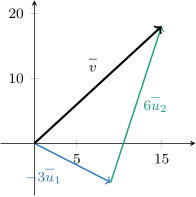
The last line prints [1] -3 6, the entries of the vector of unknowns in order: $x = -3$ and $y = 6$ . Both equations check: $-3(-3) + 6 = 15$ and $2(-3) + 4(6) = 18$ . With columns $\overline{\vphantom{b}u}_1 = \left(\begin{smallmatrix} -3\\2 \end{smallmatrix}\right)$ and $\overline{\vphantom{b}u}_2 = \left(\begin{smallmatrix} 1\\4 \end{smallmatrix}\right)$ , the solution says $-3\overline{\vphantom{b}u}_1 + 6\overline{\vphantom{b}u}_2 = \overline{\vphantom{b}v}$ . In the figure, the vector $-3\overline{\vphantom{b}u}_1 = \left(\begin{smallmatrix} 9\\-6 \end{smallmatrix}\right)$ runs from the origin, and $6\overline{\vphantom{b}u}_2 = \left(\begin{smallmatrix} 6\\24 \end{smallmatrix}\right)$ starts at its tip and ends at $\overline{\vphantom{b}v} = \left(\begin{smallmatrix} 15\\18 \end{smallmatrix}\right)$ .

Example 12

Solve the bomber tasking of Example 4 in R, and interpret the solution:

\begin{pmatrix*}[r] 8 & 12 \\ 16 & 8 \end{pmatrix*}\begin{pmatrix*}[r] x \\ y \end{pmatrix*} = \begin{pmatrix*}[r] 28 \\ 40 \end{pmatrix*}.

ShowHide solution

Define the matrix from the two sortie loads, define the target vector, and solve:

U = matrix(c(8, 16, 12, 8), nrow = 2, ncol = 2)
v = c(28, 40)
solve(U, v)

The last line prints [1] 2 1: $x = 2$ and $y = 1$ . Two B-1B sorties and one B-52H sortie fill the tasking, because $8(2) + 12(1) = 28$ missiles and $16(2) + 8(1) = 40$ bombs.

Example 13

Solve the matrix equation of Example 1 in R:

\begin{pmatrix*}[r] 4 \\ -1 \\ 3 \end{pmatrix*} = \begin{pmatrix*}[r] 1 & 4 & 5 \\ -2 & 8 & 1 \\ 1 & -7 & 0 \end{pmatrix*}\begin{pmatrix*}[r] x_1 \\ x_2 \\ x_3 \end{pmatrix*}.

ShowHide solution

Solve as in Example 11, with the matrix built from its three columns stored as vectors.

u1 = c(1, -2, 1)
u2 = c(4, 8, -7)
u3 = c(5, 1, 0)
U = matrix(c(u1, u2, u3), nrow = 3, ncol = 3)
v = c(4, -1, 3)
solve(U, v)

The last line prints [1] -1.0975610 -0.5853659 1.4878049: $x_1 \approx -1.098$ , $x_2 \approx -0.585$ , and $x_3 \approx 1.488$ .

Example 14

Solve the system of Example 8 in R:

\begin{aligned} 4x &= 7 - 2y + z \\ y - 3z &= x + 1 \\ 5z &= 2x. \end{aligned}

ShowHide solution

The matrix equation, from Example 8, is

\begin{pmatrix*}[r] 4 & 2 & -1 \\ -1 & 1 & -3 \\ -2 & 0 & 5 \end{pmatrix*}\begin{pmatrix*}[r] x \\ y \\ z \end{pmatrix*} = \begin{pmatrix*}[r] 7 \\ 1 \\ 0 \end{pmatrix*}.

Its entries go in column by column: the coefficients of $x$ , then of $y$ , then of $z$ .

U = matrix(c(4, -1, -2, 2, 1, 0, -1, -3, 5), nrow = 3, ncol = 3)
v = c(7, 1, 0)
solve(U, v)

The last line prints [1] 0.625 2.375 0.250: $x = 0.625$ , $y = 2.375$ , and $z = 0.25$ .

Example 15

Solve the matrix equation of MMAC Question 8 in R:

\begin{pmatrix*}[r] 1 \\ 4 \\ 5 \\ 7 \end{pmatrix*} = \begin{pmatrix*}[r] -1 & 1 & -5 & 2 \\ 0 & 1 & 7 & -1 \\ 2 & 1 & 3 & -2 \\ 7 & 1 & 1 & 0 \end{pmatrix*}\begin{pmatrix*}[r] x_1 \\ x_2 \\ x_3 \\ x_4 \end{pmatrix*}.

ShowHide solution

Solve as in Example 11, entering the 16 entries column by column.

U = matrix(c(-1, 0, 2, 7, 1, 1, 1, 1, -5, 7, 3, 1, 2, -1, -2, 0), nrow = 4, ncol = 4)
v = c(1, 4, 5, 7)
solve(U, v)

The last line prints [1] 0.5783133 2.8313253 0.1204819 -0.3253012: $x_1 \approx 0.578$ , $x_2 \approx 2.831$ , $x_3 \approx 0.120$ , and $x_4 \approx -0.325$ .

Target vector first. Putting the target vector first makes R read the vector as the matrix. With $U$ and $\overline{\vphantom{b}v}$ of Example 15, R stops because a $4 \times 1$ vector is not square. In the message, a is R’s name for the first input of solve():

> solve(v, U)
Error in solve.default(v, U) : 'a' (4 x 1) must be square

Matrix not square. A matrix that is not square also stops solve(), even when the system has a solution. The system of Example 10 has the solution $a = 3$ and $b = -1$ , because $2(3) + (-1) = 5$ , $-3(-1) = 3$ , and $4(3) + 5(-1) = 7$ , and R still stops:

> B = matrix(c(2, 0, 4, 1, -3, 5), nrow = 3, ncol = 2)
> w = c(5, 3, 7)
> solve(B, w)
Error in solve.default(B, w) : 'a' (3 x 2) must be square

Singular matrix. A square matrix whose second column is a multiple of the first stops solve() as well:

> U = matrix(c(1, 2, 2, 4), nrow = 2, ncol = 2)
> v = c(1, 2)
> solve(U, v)
Error in solve.default(U, v) :
Lapack routine dgesv: system is exactly singular: U[2,2] = 0

The word singular in the message means that the matrix equation does not have exactly one solution. Here every linear combination of the columns is a multiple of the first column, because the second column is 2 times the first:

x\begin{pmatrix*}[r] 1 \\ 2 \end{pmatrix*} + y\begin{pmatrix*}[r] 2 \\ 4 \end{pmatrix*} = (x + 2y)\begin{pmatrix*}[r] 1 \\ 2 \end{pmatrix*}.

The target vector $\left(\begin{smallmatrix} 1\\2 \end{smallmatrix}\right)$ is $(x + 2y)\left(\begin{smallmatrix} 1\\2 \end{smallmatrix}\right)$ whenever $x + 2y = 1$ , and infinitely many pairs, such as $x = 1$ with $y = 0$ and $x = -1$ with $y = 1$ , satisfy that equation.

Lesson map